Handling missing data is a crucial step in data preprocessing. When working with real-world datasets, missing values are common due to various reasons such as data entry errors, sensor malfunctions, or incomplete surveys. If not handled properly, missing data can lead to biased results and reduced accuracy in machine learning models.
Ignoring missing data can lead to biased results and inaccurate predictions. There are several methods to handle missing data including imputation, deletion, and prediction. Imputation involves replacing missing values with estimated ones based on existing data, while deletion simply removes observations with missing values. Prediction uses machine learning algorithms to predict missing values based on other features in the dataset. Each method has its own advantages and limitations, so choosing the appropriate approach depends on the nature of the data and the research question at hand. Overall, handling missing data effectively is essential for building reliable and accurate machine learning models.
When it comes to dealing with missing data in your dataset, there are a few popular methods that can help you out. One approach is Multiple Imputation by Chained Equations (MICE), which fills in missing values by generating multiple imputed datasets and combining them for more accurate results. Another option is K-Nearest Neighbors (KNN) Imputation, where missing values are replaced by the average of their nearest neighbors based on similarities in other features. And finally, there’s interpolation, which estimates missing values based on existing data points using linear or curve fitting techniques. Each method has its pros and cons, so it’s important to carefully consider which one is best suited for your specific dataset and analysis goals.
MICE (Multiple Imputation by Chained Equations)
MICE is a powerful technique for handling missing values by imputing them multiple times using different models. Instead of filling in missing values with a single number, MICE creates multiple imputed datasets and then combines them for better accuracy. MICE works by predicting missing values iteratively. It starts by filling missing values with mean or median values, then builds a regression model for each variable with missing values, using other available variables as predictors.
Basically, it’s a method used in statistics to deal with missing data in a dataset. Instead of just throwing out incomplete observations, MICE fills in the missing values by creating multiple sets of plausible values through an iterative process. Each variable with missing data is imputed using other variables in the dataset, hence the term “chained equations.” This approach allows for more accurate and reliable estimates compared to simpler techniques like mean imputation or listwise deletion. MICE is especially useful when dealing with complex datasets where missingness is not completely random, making it a valuable tool for researchers looking to make the most out of their data.
import pandas as pd
import numpy as np
from fancyimpute import IterativeImputer

# Creating a dataset with missing values
data = pd.DataFrame({
    'Age': [25, np.nan, 35, 45, np.nan, 50],
    'Salary': [50000, 60000, np.nan, 80000, 90000, np.nan]
})

# Applying MICE Imputation
imputer = IterativeImputer()
data_imputed = imputer.fit_transform(data)

# Converting back to DataFrame
data_imputed = pd.DataFrame(data_imputed, columns=data.columns)
print(data_imputed)
In this code:
- We import necessary libraries: pandas, numpy, and IterativeImputer from fancyimpute.
- A dataset with missing values is created.
- The IterativeImputer is applied to predict missing values using regression models.
- The imputed dataset is converted back to a DataFrame and displayed.
Output
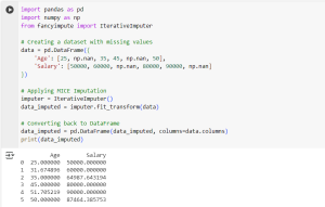
The missing values in Age and Salary are imputed using regression techniques, resulting in more accurate estimations based on existing data patterns.
KNN Imputation
K-Nearest Neighbors (KNN) imputation fills in missing values using the average of the ‘k’ nearest neighbors. The idea is that similar data points (neighbors) have similar values. KNN works well when data points are closely related. It calculates distances between data points and assigns missing values based on the nearest ones.
It’s a handy technique used in machine learning to fill in missing values by looking at the most similar data points and borrowing their values. The KNN stands for “K-nearest neighbors,” which basically means it’s going to find the closest data points to the one with missing info and use their values to make an educated guess about what the missing value should be. Pretty cool, right? It’s like having a virtual detective that can piece together the puzzle of your dataset even when there are some pieces missing.
from sklearn.impute import KNNImputer

# Creating a dataset with missing values
data = pd.DataFrame({
    'Age': [25, np.nan, 35, 45, np.nan, 50],
    'Salary': [50000, 60000, np.nan, 80000, 90000, np.nan]
})

# Applying KNN Imputation
imputer = KNNImputer(n_neighbors=2)
data_imputed = imputer.fit_transform(data)

# Converting back to DataFrame
data_imputed = pd.DataFrame(data_imputed, columns=data.columns)
print(data_imputed)
In this code:
- The KNNImputer from sklearn.impute is imported.
- A dataset with missing values is created.
- The KNNImputer is applied with n_neighbors=2, meaning it finds the two nearest neighbors for imputation.
- The missing values are filled based on the average of the nearest neighbors.
- The imputed dataset is displayed.
Output
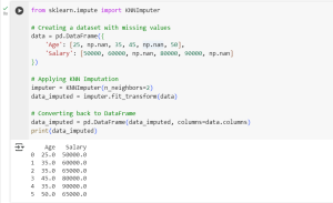
KNN finds the two nearest data points and imputes missing values by averaging them. It is useful when the data has natural clusters.
Interpolation
Interpolation estimates missing values by assuming a continuous trend in the data. It is particularly useful for time-series data where missing values can be predicted based on previous and future observations.
Basically, interpolation is the process of estimating values that are located between known data points. This can be super useful when you’re working with incomplete data sets or trying to smooth out fluctuations in your dataset. There are different methods of interpolation, such as linear, cubic spline, or nearest neighbor interpolation. Linear interpolation, for example, simply draws straight lines between two known data points to estimate the value in between. Cubic spline interpolation uses polynomial functions to create smoother curves that pass through all the data points. Nearest neighbor interpolation is the simplest method – it just takes the value of the closest known data point to estimate missing values.
# Creating a dataset with missing values
data = pd.DataFrame({'Time': [1, 2, 3, 4, 5, 6],
                     'Temperature': [30, np.nan, 32, np.nan, 34, 35]})

# Applying Interpolation
data['Temperature'] = data['Temperature'].interpolate()
print(data)
In this code:
- A dataset with missing temperature values over time is created.
- The interpolate() function is used to fill in missing values based on a linear trend.
- The missing values are estimated based on previous and next known values.
- The interpolated dataset is displayed.
Output
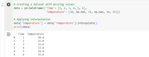
Interpolation assumes a linear trend and fills missing values accordingly. It is useful when the data follows a predictable pattern.
Conclusion
Handling missing data is essential to ensure accurate machine learning models. MICE is best for datasets with complex relationships, KNN is useful for datasets with similar patterns, and Interpolation is suitable for time-series data. Understanding these techniques will help in selecting the most appropriate method for different datasets.
Each method has its own advantages and use cases. MICE provides robust predictions when multiple variables are correlated, KNN works effectively in datasets with clusters, and interpolation is best suited for structured and continuous data. Choosing the right method depends on the nature of the dataset and the problem being solved. By effectively handling missing values, we can ensure better data quality and improve the performance of machine learning models.