Introduction: Are you eager to delve into the fascinating world of machine learning? TensorFlow, Google’s open-source library for machine learning, offers a plethora of tools and resources to help you get started. In this beginner-friendly guide, we’ll walk through the process of training TensorFlow models in Python, making it accessible for newcomers to the field. To build a predictive model that can forecast customer churn – a critical task for businesses aiming to retain their valuable clientele.

Step 1: Setting the Stage

Our adventure begins by laying the groundwork. We import the essential libraries – Pandas for data manipulation and scikit-learn for model evaluation. The dataset we’ll be working with contains valuable insights into customer behavior, stored in a CSV file named “Churn.csv”.Churn

import pandas as pd


from sklearn.model_selection import train_test_split


df = pd.read_csv("/content/Churn.csv")


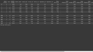
df

Output:

Step 2: Unveiling the Data

Ah, the heart of our expedition – the data itself. We use Pandas to load the dataset into a DataFrame, granting us a bird’s eye view of its contents. With a simple command, we reveal the structure of our data, gaining insights into the features and the target variable – churn.

Step 3: Preparing for the Journey

Before we can traverse the machine learning landscape, we must prepare our dataset. Utilizing Pandas’ magical “get_dummies” function, we transform categorical variables into numerical ones, a crucial step in training our model. Additionally, we encode our target variable – churn – into binary form, a 0 for ‘No’ and a 1 for ‘Yes’, simplifying our predictive task.

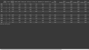
x = pd.get_dummies(df.drop(['Churn','Customer ID'],axis=1))

x

Output:

y=df['Churn'].apply(lambda x:1 if x=='Yes' else 0)

Certainly! This line of code creates a new variable called ‘y’ by applying a lambda function to the ‘Churn’ column of the DataFrame ‘df’.

The lambda function checks each value in the ‘Churn’ column. If the value is ‘Yes’, it returns 1; otherwise, it returns 0.

In essence, this line converts categorical labels (‘Yes’ and ‘No’) into numerical values (1 and 0), making it suitable for training a machine learning model, particularly for binary classification tasks.

Output:

0       0
1       0
2       0
3       1
4       0
       ..
7039    0
7040    0
7041    0
7042    1
7043    0
Name: Churn, Length: 7044, dtype: int64

Step 4: Charting Our Course

With our data primed and ready, it’s time to chart our course. We split our dataset into training and testing sets using scikit-learn’s trusty “train_test_split” function, ensuring our model’s ability to generalize to unseen data.

from sklearn.model_selection import train_test_split
x_train,x_test,y_train,y_test=train_test_split(x,y,test_size=0.2,random_state=2020)


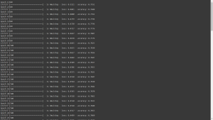
x_train

Output:

x_test

y_train

Output:

2461    0
4519    1
11      0
320     0
500     1
       ..
2139    0
3779    0
6774    1
4488    0
864     1
Name: Churn, Length: 5635, dtype: int64

y_test

Output:

6162    0
1465    0
2658    0
3470    0
4205    0
       ..
6856    0
3403    1
5253    0
688     1
878     0
Name: Churn, Length: 1409, dtype: int64

Step 5: Crafting Our Model

Ah, the moment we’ve been eagerly awaiting – model construction. We turn to TensorFlow, the master craftsman of neural networks. With its intuitive Sequential API, we assemble our model layer by layer, each one adding depth and complexity to our predictive engine. We opt for a simple yet powerful architecture – a densely connected neural network with ReLU activation functions to introduce non-linearity.

Importing TensorFlow and Keras:

import tensorflow as tf
from tensorflow import keras

We’re importing TensorFlow, a powerful library for machine learning, and specifically the Keras module, which provides a high-level interface for building neural networks.

Importing Necessary Components:

from keras.models import Sequential, load_model
from keras.layers import Dense
from sklearn.metrics import accuracy_score

Here, we’re importing specific components from Keras and scikit-learn. Sequential allows us to build a sequential model layer by layer, Dense represents a fully connected layer in our neural network, and accuracy_score from scikit-learn helps us evaluate the accuracy of our model later on.

Initializing the Model:

model = Sequential()


We’re creating a sequential model, which means we’ll be adding layers to it one by one.

Adding Layers to the Model:

model.add(Dense(units=32, input_dim=len(x_train.columns), activation="relu"))
model.add(Dense(units=64, activation="relu"))
model.add(Dense(units=1, activation="sigmoid"))

Here, we’re adding layers to our neural network model. The first layer (input_dim) expects input data with a shape corresponding to the number of features in our training data. We use Rectified Linear Unit (ReLU) activation for the hidden layers and Sigmoid activation for the output layer to ensure values between 0 and 1 for binary classification.

Compiling the Model:

model.compile(optimizer="sgd", loss="binary_crossentropy", metrics=["accuracy"])


This line compiles our model, specifying the optimizer (Stochastic Gradient Descent), loss function (Binary Crossentropy), and the metric we want to monitor during training (accuracy).

Importing NumPy for Data Manipulation:

import numpy as np


We import NumPy, a fundamental package for scientific computing with Python, to facilitate data manipulation.

Step 6: Fueling Our Model

No journey is complete without sustenance, and for our model, that means optimization. We fuel our neural network with the stochastic gradient descent (SGD) optimizer, guiding it towards minimizing the binary cross-entropy loss – a beacon illuminating the path to predictive prowess.

Step 7: Training Our Model

With our model primed and our data prepared, we embark on the training phase. Guided by TensorFlow’s graceful choreography, we dance through epochs, refining our model’s weights and biases with each step. Our model learns to discern patterns within the data, honing its predictive abilities with every iteration.

Converting x_train:

x_train = np.asarray(x_train).astype(np.float32)

This line converts the x_train data, which likely consists of features or input variables, into a NumPy array using np.asarray(). Then, .astype(np.float32) is used to ensure that the data type of the array elements is float32, which is a common data type for numerical data in machine learning models.

Converting y_train:

y_train = np.asarray(y_train).astype(np.float32)

Similarly, this line converts the y_train data, which likely represents the target variable or labels, into a NumPy array. Again, .astype(np.float32) is applied to ensure that the data type of the array elements is float32, which is suitable for classification tasks where the target variable is typically encoded as numerical values.

By converting the data to float32, we ensure consistency in data types and prepare the training data for consumption by TensorFlow’s neural network model.

model.fit(x_train,y_train,epochs=100,batch_size=32)

output:

This line initiates the training process for our neural network model (model). The fit() function takes in the training features (x_train) and the corresponding target labels (y_train) as input.

Training Parameters:

• • epochs=100: Specifies the number of times the entire training dataset will be passed forward and backward through the neural network. In this case, we’re training the model for 100 epochs.
  • batch_size=32: Defines the number of samples that will be propagated through the network at once before updating the model’s weights. Here, we’re using a batch size of 32, which is a common choice in practice.

During training, the model learns to adjust its weights and biases to minimize the specified loss function (binary cross-entropy, as defined in the model compilation step) and improve its predictive performance on the training data. Each epoch represents one complete pass through the training dataset, with the model updating its parameters after processing each batch of data.

By training the model for multiple epochs and iterating over the entire training dataset, we aim to improve the model’s accuracy and ability to generalize to unseen data.

Step 8: Navigating Uncharted Waters

As our model completes its training, we prepare to navigate uncharted waters – the testing phase. Armed with our trusty testing set, we unleash our model upon unseen data, eager to gauge its predictive prowess. With bated breath, we await the results – accuracy, our compass guiding us towards validation or recalibration.

Converting Test Data to NumPy Arrays:

x_test = np.asarray(x_test).astype(np.float32)
y_test = np.asarray(y_test).astype(np.float32)

Here, we’re converting our test data (x_test and y_test) into NumPy arrays. This conversion ensures that our data is in a suitable format for prediction by the trained model. We specify np.float32 as the data type to ensure consistency and compatibility with the model.

Making Predictions with the Model:

y_hat = model.predict(x_test)

This line uses our trained neural network model (model) to make predictions on the test data (x_test). The predict() function takes the test features as input and returns the predicted values for the target variable. In this case, y_hat contains the predicted churn probabilities for each data point in the test set.

Output:

 

Converting Probabilities to Binary Predictions:

y_hat

Output:

array([[0.49901065],
       [0.2660773 ],
       [0.38442683],
       ...,
       [0.214831  ],
       [0.56731576],
       [0.03655761]], dtype=float32)

 

y_hat = [0 if val < .5 else 1 for val in y_hat]

Here, we convert the predicted churn probabilities (y_hat) into binary predictions. For each probability value, if it’s less than 0.5, we classify it as class 0 (no churn), and if it’s greater than or equal to 0.5, we classify it as class 1 (churn). This thresholding step simplifies our predictions into a more interpretable format.

y_hat

Output:

[0,
 0,
 0,
 1,
 1,
 1,
 0,
 0,
 0,
 0,
 0,
 0,
 0,
 0,
 0,
 0,
 0,
 0,
 1,
 0,
 0,
 0,
 1,
 1,
 0,
 1,
 0,
 0,
 0,
 1,
 0,
 0,
 0,
 1,
 1,
 0,
 0,
 1,
 1,
 0,
 0,
 0,
 0,
 0,
 0,
 1,
 0,
 0,
 0,
 1,
 0,
 0,
 0,
 0,
 1,
 0,
 1,
 0,
 0,
 0,
 0,
 0,
 0,
 0,
 0,
 0,
 0,
 0,
 0,
 0,
 0,
 0,
 0,
 0,
 1,
 0,
 0,
 1,
 0,
 0,
 0,
 0,
 1,
 0,
 0,
 0,
 1,
 1,
 1,
 1,
 0,
 0,
 0,
 1,
 0,

Calculating Accuracy:

accuracy_score(y_test, y_hat)

Output:

0.8140525195173882

Finally, we calculate the accuracy of our model’s predictions compared to the true labels (y_test). The accuracy_score() function from scikit-learn measures the proportion of correctly classified data points in the test set. This metric gives us an indication of how well our model performs on unseen data, helping us evaluate its effectiveness in predicting churn.

Step 9: Celebrating Success

Victory! Our model emerges triumphant, boasting an impressive accuracy score. With a simple yet robust architecture and the power of TensorFlow at our command, we’ve successfully constructed a predictive engine capable of forecasting customer churn with remarkable precision.

Conclusion: