ARIMA time – series generator

This tutorial explores the ARIMA model for time series forecasting in Python, covering fundamentals, model building, and tuning with practical examples. It’s designed to help you effectively forecast and analyze trends in time series data.

ARIMA Model For Time Series

The steps which involved are shown below:

Step 1: Import Libraries

import pandas as pd
import matplotlib.pyplot as plt
from statsmodels.tsa.arima.model import ARIMA
from statsmodels.tsa.stattools import adfuller

Step -2: Load the Dataset

# Load the data
df = pd.read_csv('/content/Task3.csv', parse_dates=['Date'], index_col='Date')

Step -3: Visualize the data

# Visualize the data
df.plot(title='Time Series Data', ylabel='Value', xlabel='Date')
plt.show()

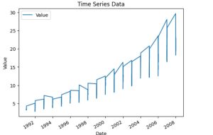
“Time series data plot showing a rising trend, used in ARIMA model forecasting analysis.”

Step 4: Check for stationarity

# Define p, d, q values (initial guesses)
p = 1  # autoregressive part
d = 1  # differencing part (0 if the data is stationary)
q = 1  # moving average part
# Check for stationarity
result = adfuller(df['Value'])
print(f'ADF Statistic: {result[0]}')
print(f'p-value: {result[1]}')

ADF Statistic: 3.14518568930673
p-value: 1.0

Step 5:  If not stationary, apply differencing

# If not stationary, apply differencing
if result[1] > 0.05:
    df['value_diff'] = df['Value'].diff().dropna()
    df['value_diff'].plot(title='Differenced Time Series Data')
    plt.show()

    # Fit ARIMA model (after differencing)
    model = ARIMA(df['value_diff'].dropna(), order=(p, d, q))
else:
    # Fit ARIMA model (no differencing needed)
    model = ARIMA(df['Value'], order=(p, d, q))

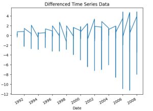
“Plot of differenced time series data showing fluctuations, used in ARIMA model preprocessing for trend removal and stationarity.”

Step 6: Fit the model and Print Summary

# Fit the model
model_fit = model.fit()
# Print model summary
print(model_fit.summary())

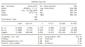
“ARIMA model summary output displaying key coefficients, standard errors, and statistical tests for time series forecasting analysis.”

Step 7: Plot diagnostics

# Plot diagnostics
model_fit.plot_diagnostics(figsize=(10, 8))
plt.show()

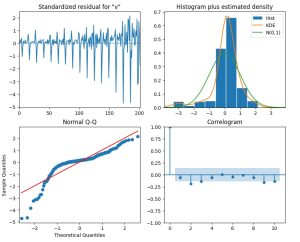
The image show a time series analysis plot, including standardized residuals, a histogram and density plot, a normal Q-Q plot, and a correlogram.

Step 8: Forecast future values

# Forecast future values
forecast = model_fit.get_forecast(steps=10)
forecast_df = forecast.conf_int()
forecast_df['Forecast'] = model_fit.predict(start=forecast_df.index[0], end=forecast_df.index[-1])
forecast_df['Value'] = df['Value'][-1]

A 10-step prediction with confidence intervals is generated and compared against the actual data in a DataFrame.

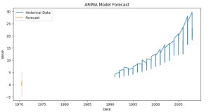
Step 9: Plot forecast

# Plot forecast
plt.figure(figsize=(10, 5))
plt.plot(df['Value'], label='Historical Data')
plt.plot(forecast_df['Forecast'], label='Forecast')
plt.fill_between(forecast_df.index, forecast_df.iloc[:, 0], forecast_df.iloc[:, 1], color='pink')
plt.legend(loc='upper left')
plt.title('ARIMA Model Forecast')
plt.xlabel('Date')
plt.ylabel('Value')
plt.show()