INTRODUCTION
There are many applicable business cases for string matching. When unique identifier does not exist for data points, there are some unstructured data to make matching possible. In our case, the unstructured data is text. For example, some can match customers, products, company data come from different data sources. Furthermore a bank can match customer informations with their social accounts.
Steps :
- Description and Loading of Dataset.
- Measuring String Similarity (Levenshtein Distance & Sorted Levenshtein Distance)
- Issues with String Matching Measures
- Feature engineering on Dataset
- Prediction of Matches with Machine Learning (Perceptron, Logistic Regression, Support Vector Machines, Multilayer Perceptron)
Examples of string matching algorithms :
A prime example of a string matching algorithm frequently used in machine learning is the “Knuth-Morris-Pratt (KMP) algorithm” which efficiently searches for a pattern within a text by pre-processing the pattern to avoid unnecessary character comparisons, making it particularly useful for tasks like text analysis and sequence matching in biological data.
-
Efficient for single pattern search :KMP excels when you need to search for a single pattern within a large text, optimizing the search process by utilizing information from previously matched characters.
-
Preprocessing step :
Before searching, the KMP algorithm constructs a “partial match table” from the pattern, allowing it to skip certain characters in the text when a mismatch occurs.
-
Rabin-Karp algorithm :
Uses hashing to quickly identify potential matches, making it useful for large datasets where checking every character combination is inefficient.
-
Levenshtein distance:
Measures the similarity between two strings by calculating the minimum number of edits required to transform one string into the other, often used in fuzzy matching scenarios.
-
Aho-Corasick algorithm:Efficiently searches for multiple patterns within a text simultaneously, useful for tasks like keyword extraction or pattern recognition.
IN-DEPTH EXPLAINATION OF EVERY COMMONLY KNOWN STRING MATCHING ALGORITHMS :
1. Knuth-Morris-Pratt or KMP :
Knuth-Morris-Pratt or KMP is a linear string matching algorithm with low time complexity of O(n+m), where n is the string length and m is the pattern length. In this article, we will what KMP algorithm is, how it works, algorithm for LPP table.KMP is a linear string-matching algorithm with low time complexity. It is the solution to the drawbacks of previous text-matching algorithms. You probably have used the advantages of the string-matching algorithm in your life. For example, while working on Microsoft applications like Microsoft Word, you might use the “Find” option to identify similar words. A pattern-matching algorithm supports the functionality of this Microsoft Word feature. In this article, we will understand the working of the KMP string-matching algorithm. We will also solve an example using the KMP algorithm.To begin with, we should first understand why the KMP algorithm was needed and what the naive string-matching algorithms had problems with.
What is the Need for the KMP Algorithm?
To match a pattern and a string an application use string-matching algorithms. The simplest algorithm is the basic or naïve string-matching algorithm.
The basic algorithms have some drawbacks and are not effective enough to be used for string-matching applications.
- The basic string-matching algorithms consume more time.
- They use back-tracking whenever there is a mismatch in the string character and a matching pattern character.
- With the increasing length of the sample pattern and original string, it is not feasible to repeat the matching process whenever there is a mismatch.
- The repeated process consumes more memory and time.
- Their time complexity is O(n*m), where n is the length of the text or string and m is the length of the pattern.
To overcome the problems with the naïve algorithm. There was a need for a fruitful and effective string-matching algorithm. This requirement gives birth to the KMP algorithm.
What is KMP Algorithm?
KMP is the fastest string-matching algorithm. Its full form is Knuth Morris Pratt Algorithm. The KMP algorithm got this name from the name of its inventors. In 1970, James H Morris, Vaughan Pratt, and Donald Knuth invented this linear string-matching algorithm.
The KMP is the only string-matching algorithm with a time complexity of O(n+m), where n is the string length and m is the pattern length.
In string-matching algorithms, there are two terminologies: sting or text and pattern.
- String or text is the original string that is used for matching.
- The pattern is the sample text which is to be matched.
Working of KMP Algorithm with an Example
In this section, we will discuss the working of the KMP algorithm with an example. In the KMP algorithm, an index number is used to track each character of the string and pattern. A variable is used to trace the index numbers.
The matching of each character of text and pattern occurs between two strings.
There is a pie table or Longest Proper Prefix (LPP) table. For making an NPP table, there are two terms known as prefixes and suffixes in a string.
There is a pie table or Longest Proper Prefix (LPP) table. For making an NPP table, there are two terms prefixes, and suffixes in a string.
For example, in a string:
a b a b
- The prefix for the above string can be: a, ab, or aba. The prefix excludes the last string character.
- The suffix for the above string can be: b, ba, or bab. It excludes the first character of the string.
Consider an example to make an LPP table.
String = ababcb
And the LPP table is shown below:
Index value: 1 2 3 4 5
| a | b | a | b | d |
| 0 | 0 | 1 | 2 | 0 |
Sample string
LLP values
- We check that, in the string the first “a” comes for the first time so its value is 0.
- “b” comes the first time in the string so its value is 0.
- The next character in the string is “a” it is already present with an index value of 1 so its value will be 1.
- The next character “b” is repeating and it is present at index value 2, so its value will be 2.
- String character “c” comes the first time in the string, so its value will be 0.
This is how you can make an LPP table by using the same index values for repeating characters.
Working of the Knuth Morris Pratt Algorithm
String = ababcabcab


We take two variables “i” and “j” respectively for the index values of the string and pattern. The value of variable j is 0. With every value of variable i, the next value of j will be used for comparison.
- When i = 1, j= 0.


- When i =2, j = 1.


- When i = 3, j = 2.


- When i = 4, j = 3.


- When i = 5, j = 4.


- So, the value of variable i = 5 and j at 5 denotes the value 0 as per LLP table value of character d. The value of variable i will increase and it does not start from the starting point like in a naïve string-matching algorithm.
- Now, i = 6, j = 0


- When i = 7, j = 1.


- When i = 8, j = 2.


- It is a mismatch at j = 2. Looking at its value in the LLP table. The value of j = 0 and i will increase to the next value.
- When i = 9, j = 0.
Comparing the next value with the “i” value.

- When i =10, j = 1.

In this way, we can match strings.
Algorithm for the LLP Table
- Take two variables i and j to trace the pattern.
- Initially, i <- 0, and j <- 2.
- Set LLP [0] = 0. The LLP value of the first character is always 0.
- if pattern [i] == pattern [j+1]
LLP [q] <- j+1
- if pattern [i]! = pattern[j+1]
LLP [q] <- 0
Step by Step Knuth Morris Pratt Algorithm
- Take two variables x and y to trace the index values of the string and pattern respectively.
- x <- 1, y <- 0, len <- length of the string.
- While x < string[len]
If string [x] == pattern [y + 1]
It is a match.
x <- x+1 and y <- y+1.
- else If string [x]!= pattern [y+1]
It is a mismatch.
x <- x+1 and y <- LLP[y]
Conclusion
The KMP algorithm is used in plagiarism, DNA sequencing, checking word spelling, and many more. It is the fastest string-matching algorithm with an O(m+n) time complexity. The KMP algorithm is a little harder to understand than the naïve algorithm.
2. Rabin-Karp algorithm :
What is Rabin-Karp Algorithm?
The Rabin-Karp algorithm is a string matching algorithm that efficiently finds patterns within a larger text using a technique called hashing.
The basic idea is to convert the pattern and each possible substring of the text into numeric values (hashes) and then compare these values rather than the strings themselves. This allows for faster comparisons, especially when dealing with large texts.
The Rabin-Karp algorithm for string matching is useful because it can quickly find patterns in large texts. It’s especially good when you need to search for multiple patterns at once or when the text is very long.
How Does Rabin-Karp Algorithm Work?
-
Hashing the Pattern: First, the algorithm turns the pattern (the word or sequence you’re looking for) into a number using a hash function. This number is like a unique ID for the pattern.
-
Hashing the Text: Next, the algorithm takes the first part of the text that is the same length as the pattern and turns it into a number using the same hash function.
-
Comparing Hashes: The algorithm compares the number (hash) of the pattern with the number (hash) of the part of the text. If the numbers are the same, it means the pattern might be there. If the numbers are different, the pattern is definitely not there.
-
Sliding the Window: If the numbers don’t match, the algorithm slides over to the next part of the text, creates a new hash for this part, and compares again. This sliding continues until the whole text is checked.
-
Collision Check: Sometimes, different parts of the text can have the same hash number even if they are not the same as the pattern. When the hash numbers match, the algorithm checks the actual text to make sure it really found the pattern.
Key Concepts to Learn
1. Hash Function
A hash function is a mathematical function that converts a string (like a sequence of characters) into a fixed-size numeric value, which is called a hash. In the Rabin-Karp algorithm, the hash function plays a crucial role by turning both the pattern and the substrings of the text into numbers that can be easily compared.
The hash function takes a string as input and returns a unique number (hash) for that string.
For example, the string “abc” might be converted to the number 294 (this is a simplified example; actual hash functions are more complex and use modular arithmetic).
By converting strings into numbers, the Rabin-Karp algorithm can compare the pattern with parts of the text much faster. Instead of comparing the strings character by character, it just compares their hash values. If the hash values match, then the strings are likely to match as well.
However, because different strings can sometimes produce the same hash (a collision), the algorithm must check the actual strings whenever a match is found.
2. Sliding Window Technique
The sliding window technique is a method used by the Rabin-Karp algorithm to move through the text efficiently while updating the hash value.
How It Works:
Imagine you have a window that covers a substring of the text that is the same length as the pattern. You start by calculating the hash for the first substring within this window. Then, you slide the window one character to the right to cover the next substring.
Instead of recalculating the hash from scratch for each new substring, the algorithm uses the hash of the previous substring and updates it by removing the effect of the first character and adding the effect of the new character.
For example, if your current window covers “abc” (with a hash of 294), and you move the window to cover “bcd”, you can quickly update the hash by subtracting the effect of ‘a’ and adding the effect of ‘d’.
This technique reduces the number of operations needed to calculate the hash for each new substring, making the algorithm much faster. Instead of recalculating the hash for every substring from scratch, you only need to make a few adjustments, which is much quicker.
Pseudocode for Rabin-Karp Algorithm
def rabin_karp(pattern, text):
    m = len(pattern)
    n = len(text)
    p_hash = hash(pattern)    # Hash value for the pattern
    t_hash = hash(text[:m])   # Hash value for the first substring of text
    base = 31                 # Base for the hash function (can be any prime number)
    h = base ** (m-1)         # Highest power of base for the length of the pattern

    for i in range(n - m + 1):
        if p_hash == t_hash:  # If hash values match
            if text[i:i+m] == pattern:  # Check the actual characters
                return i  # Pattern found at index i
        if i < n - m:
            # Calculate hash for the next substring
            t_hash = (t_hash - ord(text[i]) * h) * base + ord(text[i+m])

    return -1  # Pattern not found
Rabin-Karp Algorithm Example
Let’s walk through an example to see how the Rabin-Karp algorithm for string matching works:
- Text: “abcdef”
- Pattern: “cde”
Step 1: Compute the Hash Value of the Pattern
Let’s say hash(“cde”) = 3*31^2 + 4*31^1 + 5*31^0 = 2886.
Step 2: Compute the Hash Value of the First Substring of the Text
For the first substring “abc”:
- hash(“abc”) = 1*31^2 + 2*31^1 + 3*31^0 = 1026.
Step 3: Slide the Window Over the Text and Compare Hash Values
Slide the window to the next substring “bcd”:
- Update hash: hash(“bcd”) = (1026 – 1*31^2) * 31 + 4 = 1957.
- No match with the pattern’s hash, so slide again.
Slide to the next substring “cde”:
- Update hash: hash(“cde”) = (1957 – 2*31^2) * 31 + 5 = 2886.
- The hash matches the pattern’s hash.
Step 4: Check for Hash Collisions
Since the hash values match, we compare the actual substring “cde” with the pattern “cde”.
They match, so we’ve found the pattern at index 2 in the text.
Handling Hash Collisions in Rabin-Karp Algorithm
What is Hash Collision?
A hash collision occurs when two different strings or pieces of data produce the same hash value. Since a hash function converts strings into fixed-size numeric values, there’s a possibility that different strings could end up with the same hash.
This happens because a hash function can map many possible inputs to the same output, especially when dealing with large texts or patterns.
For example, imagine two different substrings “abc” and “xyz” that both produce the same hash value of 1234. Even though the strings are different, the hash function assigns them the same numeric ID. This situation is what we call a hash collision.
Why Do Hash Collisions Occur?
- Finite Hash Space: Since the hash function maps a potentially infinite number of input strings to a finite set of hash values, collisions are inevitable when multiple inputs produce the same output.
- Simplified Hash Functions: Basic hash functions might not be complex enough to distribute values uniformly across the possible range, increasing the chances of collisions.
How to Handle Collisions
When a hash collision occurs in the Rabin-Karp algorithm, the algorithm needs a way to ensure that it doesn’t mistakenly identify a match when the strings are actually different.
Check the Hash Values First:
The algorithm first compares the hash value of the pattern with the hash value of the current substring of the text. If the hash values don’t match, the algorithm knows that the strings are different, and it moves on to the next substring.
Perform a Direct String Comparison:
If the hash values match, the algorithm recognizes that there could be a collision, meaning the two strings might not actually be the same.
- To resolve this, the algorithm performs a direct comparison of the pattern and the current substring character by character.
- If the characters match, the pattern is found in the text.
- If the characters do not match, the algorithm identifies the situation as a hash collision and continues searching by sliding the window to the next substring.
Example:
- Suppose the pattern is “abc” and the text contains a substring “xyz” that has the same hash value as “abc”.
- The algorithm first notices that the hash values match and then checks the actual strings.
- Upon comparing “abc” with “xyz”, it realizes that they are different, so it moves on without considering it a match.
Time Complexity of Rabin-Karp Algorithm
|
Scenario |
Time Complexity |
Explanation |
|
Best Case |
O(n + m) |
In the best case, there are no hash collisions, and each substring is checked once. Hash calculations and comparisons are done in linear time. |
|
Average Case |
O(n + m) |
On average, the algorithm efficiently computes hashes and performs only a few character comparisons, leading to linear time complexity. |
|
Worst Case |
O(n * m) |
In the worst case, there are many hash collisions, requiring direct comparison of the pattern with multiple substrings, leading to a quadratic time complexity. This can happen if the hash function is poor or if the text contains many similar substrings. |
- n: Length of the text.
- m: Length of the pattern.
Space Complexity of Rabin-Karp Algorithm
|
Component |
Space Complexity |
Explanation |
|
Hash Values |
O(1) |
The space required to store the hash value of the pattern and the current substring is constant. Only a few variables are needed, regardless of the size of the text or pattern. |
|
Pattern |
O(m) |
The space needed to store the pattern itself is proportional to its length. This is required for direct comparison in case of hash collisions. |
|
Sliding Window |
O(m) |
The space needed for the sliding window (current substring) is also proportional to the pattern’s length, as only one substring is processed at a time. |
|
Total Space |
O(m) |
Overall, the algorithm requires space proportional to the length of the pattern. The additional space for hash values and other variables is constant and does not depend on the text size. |
Advantages of Rabin-Karp Algorithm
- Efficient for Multiple Patterns: Particularly effective when searching for multiple patterns in a text simultaneously.
- Fast Hash-Based Comparisons: Uses hashing to quickly compare substrings, making it faster than brute-force methods in average cases.
- Simple to Implement: The algorithm is relatively easy to understand and implement with basic hashing techniques.
- Good for Exact Matches: Works well when exact pattern matching is required, as hash comparisons are quick.
Limitations of Rabin-Karp Algorithm
- Hash Collisions: Can lead to false positives, requiring additional string comparisons, which slows down the process.
- Poor Worst-Case Performance: In the worst case, with many hash collisions, it can degrade to O(n * m) time complexity, similar to a brute-force approach.
- Sensitive to Hash Function: The efficiency heavily depends on the choice of a good hash function. Poor hash functions increase the likelihood of collisions.
- Limited to Exact Matching: Not suitable for approximate or fuzzy matching, as it relies on exact hash value comparisons.
Applications of Rabin-Karp Algorithm
- Text Searching: Efficiently finds occurrences of a pattern in large bodies of text, such as searching for keywords in documents or databases.
- Plagiarism Detection: Compares large blocks of text across different documents to detect copied content.
- DNA Sequence Analysis: Used in bioinformatics to match DNA or protein sequences, identifying specific patterns within biological data.
- Digital Forensics: Helps in identifying patterns or sequences in digital files for forensic analysis.
- Network Security: Detects malicious patterns or signatures in network packets to prevent security breaches.
- Spam Filtering: Matches specific patterns or keywords in emails to filter out spam.
- Data Deduplication: Identifies duplicate patterns or sequences in data, useful in reducing storage redundancy.
- Music and Video Recognition: Recognizes patterns in audio or video files for content identification applications like Shazam.
3. Aho-Corasick Algorithm for Pattern Searching :
Given an input text and an array of k words, arr[], find all occurrences of all words in the input text. Let n be the length of text and m be the total number of characters in all words, i.e. m = length(arr[0]) + length(arr[1]) + … + length(arr[k-1]). Here k is total numbers of input words.
Example:
Input: text = "ahishers"
       arr[] = {"he", "she", "hers", "his"}

Output:
   Word
his
 appears from 1 to 3
   Word
he
 appears from 4 to 5
   Word
she
 appears from 3 to 5
   Word
hers
appears from 4 to 7
If we use a linear time searching algorithm like KMP, then we need to one by one search all words in text[]. This gives us total time complexity as O(n + length(word[0]) + O(n + length(word[1]) + O(n + length(word[2]) + … O(n + length(word[k-1]). This time complexity can be written as O(n*k + m).
Aho-Corasick Algorithm finds all words in O(n + m + z) time where z is total number of occurrences of words in text. The Aho–Corasick string matching algorithm formed the basis of the original Unix command fgrep.
- Preprocessing : Build an automaton of all words in arr[] The automaton has mainly three functions:
Go To :   This function simply follows edges
          of Trie of all words in arr[]. It is
          represented as 2D array
g[][]
where
          we store next state for current state
          and character.

Failure : This function stores all edges that are
          followed when current character doesn't
          have edge in Trie.  It is represented as
          1D array
f[]
 where we store next state for
          current state.

Output :  Stores indexes of all words that end at
          current state. It is represented as 1D
          array
o[]
 where we store indexes
          of all matching words as a bitmap for
          current state.
- Matching : Traverse the given text over built automaton to find all matching words.
Preprocessing:
- We first Build a Trie (or Keyword Tree) of all words.
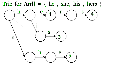
Trie
- This part fills entries in goto g[][] and output o[].
- Next we extend Trie into an automaton to support linear time matching.
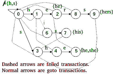
- This part fills entries in failure f[] and output o[].
Go to :
We build Trie. And for all characters which don’t have an edge at root, we add an edge back to root.
Failure :
For a state s, we find the longest proper suffix which is a proper prefix of some pattern. This is done using Breadth First Traversal of Trie.
Output :
For a state s, indexes of all words ending at s are stored. These indexes are stored as bitwise map (by doing bitwise OR of values). This is also computing using Breadth First Traversal with Failure.
Below is the implementation of Aho-Corasick Algorithm :
// C++ program for implementation of Aho Corasick algorithm
// for string matching
using namespace std;
#include <bits/stdc++.h>

// Max number of states in the matching machine.
// Should be equal to the sum of the length of all keywords.
const int MAXS = 500;

// Maximum number of characters in input alphabet
const int MAXC = 26;

// OUTPUT FUNCTION IS IMPLEMENTED USING out[]
// Bit i in this mask is one if the word with index i
// appears when the machine enters this state.
int out[MAXS];

// FAILURE FUNCTION IS IMPLEMENTED USING f[]
int f[MAXS];

// GOTO FUNCTION (OR TRIE) IS IMPLEMENTED USING g[][]
int g[MAXS][MAXC];

// Builds the string matching machine.
// arr -   array of words. The index of each keyword is important:
//         "out[state] & (1 << i)" is > 0 if we just found word[i]
//         in the text.
// Returns the number of states that the built machine has.
// States are numbered 0 up to the return value - 1, inclusive.
int buildMatchingMachine(string arr[], int k)
{
    // Initialize all values in output function as 0.
    memset(out, 0, sizeof out);

    // Initialize all values in goto function as -1.
    memset(g, -1, sizeof g);

    // Initially, we just have the 0 state
    int states = 1;

    // Construct values for goto function, i.e., fill g[][]
    // This is same as building a Trie for arr[]
    for (int i = 0; i < k; ++i)
    {
        const string &word = arr[i];
        int currentState = 0;

        // Insert all characters of current word in arr[]
        for (int j = 0; j < word.size(); ++j)
        {
            int ch = word[j] - 'a';

            // Allocate a new node (create a new state) if a
            // node for ch doesn't exist.
            if (g[currentState][ch] == -1)
                g[currentState][ch] = states++;

            currentState = g[currentState][ch];
        }

        // Add current word in output function
        out[currentState] |= (1 << i);
    }

    // For all characters which don't have an edge from
    // root (or state 0) in Trie, add a goto edge to state
    // 0 itself
    for (int ch = 0; ch < MAXC; ++ch)
        if (g[0][ch] == -1)
            g[0][ch] = 0;

    // Now, let's build the failure function

    // Initialize values in fail function
    memset(f, -1, sizeof f);

    // Failure function is computed in breadth first order
    // using a queue
    queue<int> q;

     // Iterate over every possible input
    for (int ch = 0; ch < MAXC; ++ch)
    {
        // All nodes of depth 1 have failure function value
        // as 0. For example, in above diagram we move to 0
        // from states 1 and 3.
        if (g[0][ch] != 0)
        {
            f[g[0][ch]] = 0;
            q.push(g[0][ch]);
        }
    }

    // Now queue has states 1 and 3
    while (q.size())
    {
        // Remove the front state from queue
        int state = q.front();
        q.pop();

        // For the removed state, find failure function for
        // all those characters for which goto function is
        // not defined.
        for (int ch = 0; ch <= MAXC; ++ch)
        {
            // If goto function is defined for character 'ch'
            // and 'state'
            if (g[state][ch] != -1)
            {
                // Find failure state of removed state
                int failure = f[state];

                // Find the deepest node labeled by proper
                // suffix of string from root to current
                // state.
                while (g[failure][ch] == -1)
                      failure = f[failure];

                failure = g[failure][ch];
                f[g[state][ch]] = failure;

                // Merge output values
                out[g[state][ch]] |= out[failure];

                // Insert the next level node (of Trie) in Queue
                q.push(g[state][ch]);
            }
        }
    }

    return states;
}

// Returns the next state the machine will transition to using goto
// and failure functions.
// currentState - The current state of the machine. Must be between
//                0 and the number of states - 1, inclusive.
// nextInput - The next character that enters into the machine.
int findNextState(int currentState, char nextInput)
{
    int answer = currentState;
    int ch = nextInput - 'a';

    // If goto is not defined, use failure function
    while (g[answer][ch] == -1)
        answer = f[answer];

    return g[answer][ch];
}

// This function finds all occurrences of all array words
// in text.
void searchWords(string arr[], int k, string text)
{
    // Preprocess patterns.
    // Build machine with goto, failure and output functions
    buildMatchingMachine(arr, k);

    // Initialize current state
    int currentState = 0;

    // Traverse the text through the built machine to find
    // all occurrences of words in arr[]
    for (int i = 0; i < text.size(); ++i)
    {
        currentState = findNextState(currentState, text[i]);

        // If match not found, move to next state
        if (out[currentState] == 0)
             continue;

        // Match found, print all matching words of arr[]
        // using output function.
        for (int j = 0; j < k; ++j)
        {
            if (out[currentState] & (1 << j))
            {
                cout << "Word " << arr[j] << " appears from "
                     << i - arr[j].size() + 1 << " to " << i << endl;
            }
        }
    }
}

// Driver program to test above
int main()
{
    string arr[] = {"he", "she", "hers", "his"};
    string text = "ahishers";
    int k = sizeof(arr)/sizeof(arr[0]);

    searchWords(arr, k, text);

    return 0;
}
Output
Word his appears from 1 to 3
Word he appears from 4 to 5
Word she appears from 3 to 5
Word hers appears from 4 to 7
Time Complexity: O(n + l + z), where ‘n’ is the length of the text, ‘l’ is the length of keywords, and ‘z’ is the number of matches.
Auxiliary Space: O(l * q), where ‘q’ is the length of the alphabet since that is the maximum number of children a node can have.
Applications:
? Detecting plagiarism
? Text mining
? Bioinformatics
? Intrusion Detection
CONCLUSION :
When someone says, How do I know which of the given names are same or Different? Now and then we encounter a problem where we need to have a confidence score that can help us determine whether the two given sets of string match each other or not.
Well, some here are some algorithms try to find a match based on a pattern between the two strings, or there can be another set of algorithms that just find how similar the given string /name is. Examples for the former case includes algorithm such as Naïve algorithm, KMP(Knuth-Morris-Pratt), BMH(Boyer-Moore-Horspool), etc whereas examples of the latter case include Fuzzy Matching, N-grams, Cosine Similarity, Text distance, etc.
String comparison algorithms are used to determine the similarity or difference between two or more strings. These algorithms are widely used in natural language processing, text mining, and information retrieval.
A string matching algorithm is a computational method used to find specific patterns within a larger text string, essentially identifying where a given “pattern” appears within a “text” by comparing characters at each position, with the goal of efficiently locating all occurrences of that pattern; popular examples include the Naive algorithm, Knuth-Morris-Pratt (KMP), Boyer-Moore, and Rabin-Karp, each with different strategies to optimize the search process based on the pattern and text characteristics.
-
Basic concept:
Compare characters of a pattern string against characters in a text string, sliding the pattern along the text until a match is found or the end of the text is reached.
-
Common algorithms:
- Naive algorithm: Simple, checks each character of the pattern against the text sequentially, but can be slow for large patterns.
- Knuth-Morris-Pratt (KMP): Preprocesses the pattern to efficiently jump ahead when a mismatch occurs, improving performance compared to naive approach.
- Boyer-Moore: Starts matching from the last character of the pattern and uses a “bad character heuristic” to skip large portions of the text when a mismatch is found, generally considered very fast.
- Rabin-Karp: Uses hashing to quickly check potential matches, reducing comparisons by filtering out unlikely candidates.
- Naive algorithm: Simple, checks each character of the pattern against the text sequentially, but can be slow for large patterns.
-
Applications:
Text editors (search functionality), web search engines, plagiarism detection, bioinformatics sequence analysis, network intrusion detection systems.