Have you ever considered why PyTorch is such a favorite for building neural networks? It’s not just because it has a clean and easy-to-read syntax! PyTorch makes it fun and accessible for everyone, whether you’re just starting or a seasoned machine learning pro. Let’s take a closer look at how PyTorch helps you create a simple neural network in a way that feels both effortless and powerful! In this tutorial, we will learn to build a simple neural network using PyTorch to classify handwritten digits from this MNIST dataset.
Why PyTorch is important for Neural Networks?
PyTorch is an open-source machine learning framework that uses the Python programming language and the Torch library. It is popular for building deep neural networks and is a preferred choice for deep learning research. This framework is designed to make it easier and faster to go from developing research prototypes to deploying them in real applications. PyTorch also supports over 200 different mathematical operations, making it highly versatile for various tasks.
1. Setting up the environment
1. Install Python:
The first step is to ensure Python is installed. You can download it from http://python.org.
2. Install PyTorch:
by using the following command you can install PyTorch via the pip PyTorch website
pip install torch torchvision torchaudio
Note:
Choose the appropriate command based on your system and CUDA support from the above PyTorch official website.
import os
import pandas as pd
from PIL import Image
import torch
from torch.utils.data import Dataset, DataLoader
from torchvision import transforms
import torch.nn as nn
import torch.optim as optim
import matplotlib.pyplot as plt
import torch.nn.functional as F
import numpy as np
Explanation:
- os : for file and directory operations.
- pandas : To load and process the CSV dataset.
- pillow(Image) : To load and manipulate images.
- torch and torch.nn : for building the neural network.
- torch.optim : For optimization algorithms.
- torchvision. transforms : To apply transformations.
- matplotlib.pyplot : For visualizing results
3. Load the Dataset :
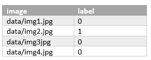
Let us assume that my dataset contains columns image_path and label ina CSV format.
Example CSV:
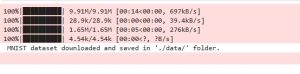
Code to Download and Load dataset
transform = transforms.Compose([
transforms.ToTensor(), # Convert images to PyTorch tensors
transforms.Normalize((0.1307,), (0.3081,)) # Normalize with mean & std
])
# Load training and test dataset
train_df = datasets.MNIST(root="./data", train=True, transform=transform, download=True)
test_df = datasets.MNIST(root="./data", train=False, transform=transform, download=True)
Output:
# Define transformations (convert images to tensors & normalize)
transform = transforms.Compose([
     transforms.ToTensor(), # Convert images to PyTorch tensors
     transforms.Normalize((0.1307,), (0.3081,)) # Normalize with mean & std
])

# Load training and test dataset
train_df = datasets.MNIST(root="./data", train=True, transform=transform, download=True)
test_df = datasets.MNIST(root="./data", train=False, transform=transform, download=True)

# Create DataLoaders (batch data loading)
train_loader = DataLoader(dataset=train_df, batch_size=64, shuffle=True)
test_loader = DataLoader(dataset=test_df, batch_size=64, shuffle=False)
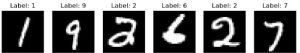
Step 2: Visualize Sample Images:
let’s visualize some images of our dataset before training:
# Get one batch of images
images, labels = next(iter(train_loader))

# Convert tensor to numpy for visualization
images = images.numpy()

# Plot the first 6 images
fig, axes = plt.subplots(1, 6, figsize=(10, 3))
for i in range(6):
    axes[i].imshow(images[i][0], cmap="gray")
    axes[i].set_title(f"Label: {labels[i].item()}")
    axes[i].axis("off")

plt.show()
Output:
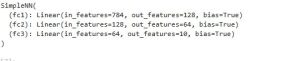
Step 3: Define the Neural Network :
now train our neural network
# Define the neural network
class SimpleNN(nn.Module):
def __init__(self):
super(SimpleNN, self).__init__()
self.fc1 = nn.Linear(28*28, 128) # Input layer (28x28 pixels -> 128 neurons)
self.fc2 = nn.Linear(128, 64) # Hidden layer (128 neurons -> 64 neurons)
self.fc3 = nn.Linear(64, 10) # Output layer (64 neurons -> 10 classes)

def forward(self, x):
x = x.view(-1, 28*28) # Flatten the image
x = F.relu(self.fc1(x)) # Apply ReLU activation
x = F.relu(self.fc2(x))
x = self.fc3(x) # Output logits
return x

# Initialize the model
model = SimpleNN()
print(model)
output:
Step 4: Define Loss Function and Optimizer :
# Define loss function (CrossEntropy for classification)
loss_function = nn.CrossEntropyLoss()

# Define optimizer (Adam optimizer)
optimizer = torch.optim.Adam(model.parameters(), lr=0.001)
Step 5: Train the Model :
device = torch.device("cuda" if torch.cuda.is_available() else "cpu")
model.to(device)

# Training loop
epochs = 5
for epoch in range(epochs):
    model.train()
    running_loss = 0.0

    for images, labels in train_loader:
        images, labels = images.to(device), labels.to(device)

        optimizer.zero_grad()
        outputs = model(images)
        loss = loss_function(outputs, labels)
        loss.backward()
        optimizer.step()

        running_loss += loss.item()

    print(f"Epoch {epoch+1}/{epochs}, Loss: {running_loss/len(train_loader):.4f}")

print("Training complete!")
output:
Epoch 1/5, Loss: 0.0304
Epoch 2/5, Loss: 0.0304
Epoch 3/5, Loss: 0.0304
Epoch 4/5, Loss: 0.0304
Epoch 5/5, Loss: 0.0304
 Training complete!
Step 6: Evaluate the Model:
model.eval()  # Set model to evaluation mode
correct = 0
total = 0

with torch.no_grad():  # Disable gradient computation
    for images, labels in test_loader:
        images, labels = images.to(device), labels.to(device)

        outputs = model(images)  # Get predictions
        _, predicted = torch.max(outputs, 1)  # Get class with highest probability
        total += labels.size(0)
        correct += (predicted == labels).sum().item()

accuracy = 100 * correct / total
print(f" Test Accuracy: {accuracy:.2f}%")
output: Test Accuracy: 97.69%
Step 7: Save and Load the Model :
# Save model
torch.save(model.state_dict(), "mnist_model.pth")
print("Model saved!")

# Load model
model = SimpleNN()
model.load_state_dict(torch.load("mnist_model.pth"))
model.eval()
Step 8: Make Predictions :
model = SimpleNN()
model.load_state_dict(torch.load("mnist_model.pth"))
model.eval()

# Test with a single image
import random
image, label = test_dataset[random.randint(0, len(test_dataset))]

# Show the image
plt.imshow(image[0], cmap="gray")
plt.title(f"Actual Label: {label}")
plt.show()

# Predict
image = image.view(-1, 28*28)  # Flatten the image
output = model(image)
_, predicted_label = torch.max(output, 1)
print(f"Predicted Label: {predicted_label.item()}")
Final output :
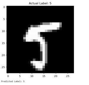
predicted Label: 5