What is Convolution Neural Network
A Convolutional Neural Network (CNN) is a type of Deep Learning neural network architecture commonly used in Computer Vision. Computer vision is a field of Artificial Intelligence that enables a computer to understand and interpret the image or visual data.
When it comes to Machine Learning, Artificial Neural Networks perform really well. Neural Networks are used in various datasets like images, audio, and text. Different types of Neural Networks are used for different purposes, for example for predicting the sequence of words we use Recurrent Neural Networks more precisely an LSTM, similarly for image classification we use Convolution Neural networks. In this blog, we are going to build a basic building block for CNN.
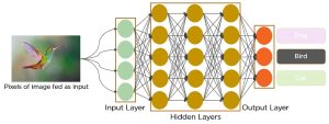
In a regular Neural Network there are three types of layers:
- Input layers: It’s the layer in which we give input to our model. The number of neurons in this layer is equal to the total number of features in our data (number of pixels in the case of an image).
- Hidden Layer: The input from the Input layer is then fed into the hidden layer. There can be many hidden layers depending on our model and data size. Each hidden layer can have different numbers of neurons which are generally greater than the number of features. The output from each layer is computed by matrix multiplication of the output of the previous layer with learnable weights of that layer and then by the addition of learnable biases followed by activation function which makes the network nonlinear.
3.Output Layer: The output from the hidden layer is then fed into a logistic function like sigmoid or softmax which converts the output of each class into the probability score of each class. CNN architecture
Convolutional Neural Network consists of multiple layers like the input layer, C C Convolutional layer, Pooling layer, and fully connected layers.
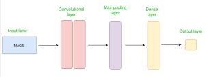
The Convolutional layer applies filters to the input image to extract features, the Pooling layer downsamples the image to reduce computation, and the fully connected layer makes the final prediction. The network learns the optimal filters through backpropagation and gradient descent.
Here is an example to show how CNN recognizes an image :
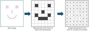
As we can see that the above diagram ,we can see that those values are lit that have a value of 1.
Layers in a Convolutional Neural Network
A convolution neural network has multiple hidden layers that help in extracting information from an image. The four important layers in CNN are:
- Convolution layer
- ReLU layer
- Pooling layer
- Fully connected layer
CONVOLUTION LAYER
This is the first step in the process of extracting valuable features from an image. A convolution layer has several filters that perform the convolution operation. Every image is considered as a matrix of pixel values.
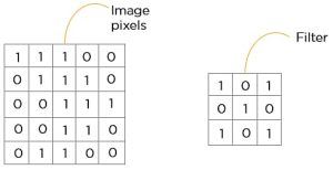
Consider the following 5×5 image whose pixel values are either 0 or 1. There’s also a filter matrix with a dimension of 3×3. Slide the filter matrix over the image and compute the dot product to get the convolved feature matrix.
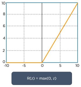
ReLU layer
ReLU stands for the rectified linear unit. Once the feature maps are extracted, the next step is to move them to a ReLU layer.
ReLU performs an element-wise operation and sets all the negative pixels to 0. It introduces non-linearity to the network, and the generated output is a rectified feature map. Below is the graph of a ReLU function:
The original image is scanned with the multiple convolutions and ReLU layers for locating the features:
1.Import Libraries:
import tensorflow as tf

from tensorflow.keras
import datasets, layers, models
import matplotlib.pyplot as plt
import numpy as np
2.Load the Data set:
(X_train, y_train), (X_test,y_test) = datasets.cifar10.load_data()
X_train.shape
Output:
(50000, 32, 32, 3)
X_test.shape
Output:
(10000, 32, 32, 3)
y_train.shape
Output:
(50000, 1)
y_train[:5]
Output:
array([[6],
[9],
[9],
[4],
[1]], dtype=uint8)
y_train is a 2D array, for our classification having 1D array is good enough.
so we will convert this to now 1D array.
y_train = y_train.reshape(-1,)
y_train[:5] Output: array([6, 9, 9, 4, 1], dtype=uint8) y_test = y_test.reshape(-1,) classes = ["airplane","automobile","bird","cat","deer","dog","frog","horse","ship","truck"] Let's plot some Images: def plot_sample(X, y, index):
plt.figure(figsize = (15,2))
plt.imshow(X[index])
plt.xlabel(classes[y[index]]) plot_sample(X_train, y_train, 0) Output: 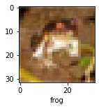
plot_sample(X_train, y_train, 1) Output: 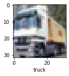
Normalizing the training data
X_train = X_train / 255.0
X_test = X_test / 255.0
Build simple artificial neural network for image classification
ann = models.Sequential([
        layers.Flatten(input_shape=(32,32,3)),
        layers.Dense(3000, activation='relu'),
        layers.Dense(1000, activation='relu'),
        layers.Dense(10, activation='softmax')
    ])

ann.compile(optimizer='SGD',
              loss='sparse_categorical_crossentropy',
              metrics=['accuracy'])

ann.fit(X_train, y_train, epochs=5)
Output:
Epoch 1/5
1563/1563 [==============================] - 2s 2ms/step - loss: 1.8074 - accuracy: 0.3561
Epoch 2/5
1563/1563 [==============================] - 2s 1ms/step - loss: 1.6208 - accuracy: 0.4285
Epoch 3/5
1563/1563 [==============================] - 2s 2ms/step - loss: 1.5380 - accuracy: 0.4585
Epoch 4/5
1563/1563 [==============================] - 2s 2ms/step - loss: 1.4808 - accuracy: 0.4806
Epoch 5/5
1563/1563 [==============================] - 2s 2ms/step - loss: 1.4326 - accuracy: 0.4928
We can see that the accuracy around 49%.
from sklearn.metrics import confusion_matrix , classification_report
import numpy as np
y_pred = ann.predict(X_test)
y_pred_classes = [np.argmax(element) for element in y_pred]

print("Classification Report: \n", classification_report(y_test, y_pred_classes))
Out [ ]:
Classification Report:
               precision    recall  f1-score   support

           0       0.63      0.45      0.53      1000
           1       0.72      0.46      0.56      1000
           2       0.33      0.46      0.39      1000
           3       0.36      0.25      0.29      1000
           4       0.44      0.37      0.40      1000
           5       0.34      0.46      0.39      1000
           6       0.56      0.47      0.51      1000
           7       0.39      0.67      0.50      1000
           8       0.64      0.60      0.62      1000
           9       0.59      0.53      0.55      1000

    accuracy                           0.47     10000
   macro avg       0.50      0.47      0.47     10000
weighted avg       0.50      0.47      0.47     10000
Now let us build a convolutional neural network to train Our images
cnn = models.Sequential([
    layers.Conv2D(filters=32, kernel_size=(3, 3), activation='relu', input_shape=(32, 32, 3)),
    layers.MaxPooling2D((2, 2)),

    layers.Conv2D(filters=64, kernel_size=(3, 3), activation='relu'),
    layers.MaxPooling2D((2, 2)),

    layers.Flatten(),
    layers.Dense(64, activation='relu'),
    layers.Dense(10, activation='softmax')
])


cnn.compile(optimizer='adam',
              loss='sparse_categorical_crossentropy',
              metrics=['accuracy'])


cnn.fit(X_train, y_train, epochs=10)
Out[ ]:
Epoch 1/10
1563/1563 [==============================] - 2s 2ms/step - loss: 1.4407 - accuracy: 0.4810
Epoch 2/10
1563/1563 [==============================] - 2s 2ms/step - loss: 1.1084 - accuracy: 0.6109
Epoch 3/10
1563/1563 [==============================] - 2s 2ms/step - loss: 0.9895 - accuracy: 0.6574
Epoch 4/10
1563/1563 [==============================] - 2s 2ms/step - loss: 0.9071 - accuracy: 0.6870
Epoch 5/10
1563/1563 [==============================] - 2s 2ms/step - loss: 0.8416 - accuracy: 0.7097
Epoch 6/10
1563/1563 [==============================] - 2s 2ms/step - loss: 0.7847 - accuracy: 0.7262
Epoch 7/10
1563/1563 [==============================] - 2s 2ms/step - loss: 0.7350 - accuracy: 0.7448
Epoch 8/10
1563/1563 [==============================] - 2s 2ms/step - loss: 0.6941 - accuracy: 0.7574
Epoch 9/10
1563/1563 [==============================] - 2s 1ms/step - loss: 0.6516 - accuracy: 0.7731
Epoch 10/10
1563/1563 [==============================] - 2s 2ms/step - loss: 0.6187 - accuracy: 0.7836
cnn.evaluate(X_test,y_test)
Out [ ]:
[0.9021560549736023, 0.7027999758720398]
y_pred = cnn.predict(X_test)
y_pred[:5]
Out [ ]:
array([[4.3996371e-04, 3.4844263e-05, 1.5558505e-03, 8.8400185e-01,
1.9452239e-04, 3.5314459e-02, 7.2777577e-02, 6.9044131e-06,
5.6417785e-03, 3.2224660e-05],
[8.1062522e-03, 5.0841425e-02, 1.2453231e-07, 5.3348430e-07,
9.1728407e-07, 1.0009186e-08, 2.8985988e-07, 1.7532484e-09,
9.4089705e-01, 1.5346886e-04],
[1.7055811e-02, 1.1841061e-01, 4.6799007e-05, 2.7727904e-02,
1.0848254e-03, 1.0896578e-03, 1.3575243e-04, 2.8652203e-04,
7.8895986e-01, 4.5202184e-02],
[3.1300801e-01, 1.1591638e-02, 1.1511055e-02, 3.9592334e-03,
7.7280165e-03, 5.6289224e-05, 2.3531138e-04, 9.4204297e-06,
6.5178138e-01, 1.1968113e-04],
[1.3230885e-05, 2.1221960e-05, 9.2594400e-02, 3.3585075e-02,
4.4722903e-01, 4.1028224e-03, 4.2241842e-01, 2.8064171e-05,
6.6392668e-06, 1.0745022e-06]], dtype=float32)
y_classes = [np.argmax(element) for element in y_pred]
y_classes[:5] Out[]: [3, 8, 8, 8, 4] y_test[:5] Out[]: array([3, 8, 8, 0, 6], dtype=uint8) plot_sample(X_test, y_test,3) Out[]: 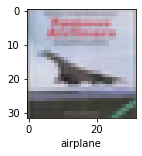
classes[y_classes[3]] Out[]: 'ship' classes[y_classes[3]] Out[]: 'ship'
Advantages of Convolutional Neural Networks (CNNs):
- Good at detecting patterns and features in images, videos, and audio signals.
- Robust to translation, rotation, and scaling invariance.
- End-to-end training, no need for manual feature extraction.
- Can handle large amounts of data and achieve high accuracy.
Disadvantages of Convolutional Neural Networks (CNNs):
- Computationally expensive to train and require a lot of memory.
- Can be prone to overfitting if not enough data or proper regularization is used.
- Requires large amounts of labeled data.
- Interpretability is limited, it’s hard to understand what the network has learned.