In this blog spot, we will explore an advanced implementation of Lasso Regression in Python using Scikit_learn. This implementation includes additional steps such as hyperparameter tuning.
What is Lasso Regression?
Lasso regression is a type of linear regression that uses shrinkage, shrinkage is where data values are shrunk towards a point, like the mean. This is a type of regression where the absolute value of the magnitude of the coefficient is used as a penalty term for the loss function. Lasso regression (Least Absolute and Selection Operator) adds a factor of the sum of the absolute value of coefficients in the optimization objective. Thus, lasso regression optimizes the following:

The objective function consists of two parts:
 : Also called residual sum of squares. This measures the sum of the squared differences between the actual and predicted values.
 : Also called Regularization term. This adds a penalty proportional to the absolute values of the coefficients, reducing some coefficients to exactly zero.
Lasso regression is a linear regression that introduces a penalty term for the magnitude of the coefficients in the model. This penalty term encourages the model to keep the coefficients as small as possible, effectively reducing the number of features upon which the given solution depends. For this reason, Lasso regression is particularly useful when dealing with high-dimensional datasets where feature selection is important.
The key characteristic of lasso regression is its ability to get some coefficients to zero, effectively excluding them from the model. This is known as feature selection and is a form of dimensionality reduction. By excluding irrelevant features, Lasso regression can improve the interpretability of the model and help prevent overfitting.
The penalty term in lasso regression is controlled by a hyperparameter, typically denoted by ‘λ’ (lambda). The larger the value of lambda ‘λ’, the greater the penalty on the coefficients, and the more coefficients will be set to zero. This makes ‘λ’ a crucial hyperparameter tp tune when using lasso regression.
Implementing Lasso Regression in Python
Let’s implement lasso regression in Python. Here’s the code:
1. Importing libraries:
The first step in any Python script is to import the necessary libraries. In this case, we’re using ‘numpy’ for numerical operations, ‘pandas’ for data manipulation, ‘scipy’ for scientific computing, ‘sklearn’ for machine learning, and ‘matplotlib’ for plotting:
import numpy as np
import pandas as pd
from scipy import stats
from sklearn.model_selection import train_test_split, GridSearchCV
from sklearn.preprocessing import StandardScaler
from sklearn.linear_model import LassoCV
from sklearn.metrics import mean_squared_error, r2_score
from sklearn.pipeline import Pipeline
from sklearn.impute import SimpleImputer
import matplotlib.pyplot as plt
2. Loading and Exploring the data:
Next, we load the dataset and perform some initial exploration. This includes checking for missing values, counting the number of features, looking at the distribution of continuous variables, and examining the correlation between different features:
#  Load the input dataset
dataset = pd.read_csv('/content/HousingData.csv')
# Explore the data
print("Missing values:", dataset.isnull().sum())
print("Number of features:", dataset.shape[1])
print("Distribution of continuous variables:")
print(dataset.describe())
print("Correlation between features:")
print(dataset.corr())
3. Outliers Detection and Removal:
After exploring the data, we detect and remove outliers using the Z-score method. The Z-score measures how many standard deviations an element is from the mean. A Z-score greater than 3 or less than -3 is usually considered to be an outlier:
# Outlier detection and removal using Z-score
z_scores = np.abs(stats.zscore(dataset))
filtered_entries = (z_scores < 3).all(axis=1)
dataset = dataset[filtered_entries]
4. Handling missing values:
Next, we handle missing values in our data by replacing them with the mean value of each feature:
numeric_transformer = Pipeline(steps=[
    ('imputer', SimpleImputer(strategy='mean')),
    ('scaler', StandardScaler())
])

preprocessor = numeric_transformer
Here is a ‘Pipeline’ object called ‘numeric_transformer’. A pipeline is a sequence of data processing elements, where the output of one element is the input of the next one. A pipeline combines steps that can be cross-validated together while setting different parameters. Here, the pipeline consists of two steps: imputation and scaling.
Imputations: This step deals with missing values in the dataset. The ‘SimpleImputer’ class provides basic strategies for imputing missing values, using the mean, median, most frequent, or constant values. Here, ‘strategy=’mean” means that missing values will be replaced with the mean values of each feature. This mean is calculated separately for each feature and only using the known values of each feature.
Scaling: This step standardizes the features by removing the mean and scaling to unit variance. This is a common requirement for many machine learning estimators: they might behave badly if the individual features do not more or less look like standard normally distributed data.
5. Splitting the Data:
We split our data into training and testing sets after preprocessing:
#  Split the data and preprocess
x = dataset.drop('Target', axis=1)
y = dataset['Target']

x_train, x_test, y_train, y_test = train_test_split(x, y, test_size=0.2, random_state=42)
6. Fitting the Model and Hyperparameter Tuning:
We then fit a Lasoo Regression model to our data and perform hyperparameter tuning using cross-validation:
#  Fit the Lasso model and choose a value for λ
lasso = LassoCV(cv=5, random_state=42)

# Create a pipeline with preprocessor and model
Pipe = Pipeline(steps=[('preprocessor', preprocessor), ('lasso', lasso)])

# Perform hyperparameter tuning
Param_grid = {
    'lasso__alphas': [np.logspace(-4, 1, 50)],
    'lasso__max_iter': [10000]
}

Grid_search = GridSearchCV(Pipe,Param_grid, cv=5,scoring='neg_mean_squared_error',n_jobs=-1)
Grid_search.fit(x_train, y_train)

print("Best Hyperparameters:",Grid_search.best_params_)
print("Optimal Lambda:", Grid_search.best_estimator_.named_steps['lasso'].alpha_)
LassoCV: ‘LassoCV’ is a lasso linear model with built-in cross-validation to find the optimal value of the alpha parameter, It’s part of the ‘sklearn.linear_model’ module. This ‘cv’ parameter determines the cross-validation splitting strategy, and ‘random-state’ is a seed used by the random number generator.
Pipeline: ‘Pipeline’ is used to assemble several steps that can be cross-validated together while setting different parameters. Here, it’s assembling the preprocessing steps and the lasso model.
GridsearchCV: ‘GridSearchCV’ is a function is ‘sklearn.model_selection’ that is used to tune the hyperparameters. It exhaustively tried every combination of the provided hyperparameter values to find the best model. Here, it finds the best values for the ‘alphas’ and ‘max_iter’ parameters of the lasso model. Here, ‘np.logspace(-4,1,50)’ generated 50 numbers spaced on a log scale between 10^-4 and 10^1. These numbers are used as candidate values for ‘alphas’ during the grid search process. ‘max_iter’ is the maximum number of iterations for the solver to converge.
Best Hyperparameters and Optimal Lambda: After fitting the gris search to the data, the best hyperparameters and the optimal lambda (alpha) are printed. ‘gris_Search.best_params_’ gives the best hyperparameters found by the grid search, and ‘grid_search.nest_estimator_.names_steps[‘lasso’].alpha_’ gives the optimal lambda(alpha) value found by cross_Validation is ‘LassoCV’.
7. Evaluating the model:
After fitting the model, we calculate the mean squared error (MSE) and R-squared value for both the training and testing sets to evaluate its performance:
# Evaluate the performance of your model
y_train_pred = Grid_search.best_estimator_.predict(x_train)
y_test_pred = Grid_search.best_estimator_.predict(x_test)

Train_mse = mean_squared_error(y_train,y_train_pred)
Test_mse = mean_squared_error(y_test,y_test_pred)
Train_r2 = r2_score(y_train,y_train_pred)
Test_r2 = r2_score(y_test,y_test_pred)

print("Train MSE:",Train_mse)
print("Test MSE:",Test_mse)
print("Train R-squared:",Train_r2)
print("Test R-squared:",Test_r2)
8. Visualizing the Results:
Finally, we visualize the actual versus predicted values using a scatter plot:
# 5. Plotting the results
plt.figure(figsize=(10, 6))

plt.scatter(y_train,y_train_pred,color='black',label='Train data')
plt.scatter(y_test,y_test_pred,color='blue',label='Test data')

Min_Val = min(min(y_train),min(y_test))
Max_Val = max(max(y_train),max(y_test))
plt.plot([Min_Val, Max_Val], [Min_Val, Max_Val],color='red',linestyle='--')

plt.title('actual vs predicted values')
plt.xlabel('actual')
plt.ylabel('predicted')
plt.legend()

plt.show()
Outputs and Evaluations:
1. Number of Features:
Output:
Number of features: 14
The dataset contains 14 features. This includes 13 independent features and 1 dependent feature ( the ‘Target’). Knowing the number of features can help you understand the dimensionality of your data.
2. Missing values:
Output:
Missing values:

Feature 1 0

Feature 2 0

Feature 3 0

Feature 4 0

Feature 5 0

Feature 6 0

Feature 7 0

Feature 8 0

Feature 9 0

Feature 10 0

Feature 11 0

Feature 12 0

Feature 13 0

Target 0
The output shows there are no missing values in your dataset for any of the features or the target variable. This is great news because if there are any gaps, those should be filled before the learning process starts, which is a complex process again.
3. Distribution of Continuous variables:
Output:
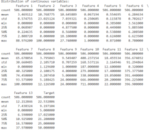
The ‘describe()’ function provides a statistical output summary of all the variables in your dataset. This includes count, mean, standard deviation, minimum value, 25th percentile, median (50th percentile), 75th percentile, and maximum values. This information help’s in understanding the range, and distribution of the data.
4. Correlation between features:
Output:
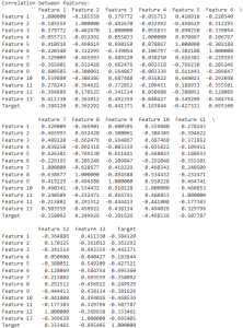
The above data shows the correlation coefficient value between all pairs of features. Correlation coefficients range from -1 to 1, with -1 indicating a perfect negative correlation, 1 indicating a perfect positive correlation, and 0 indicating no correlation. This will help you understand the relationships between features in your dataset.
5. Best Hyperparameters:
The output shows the best hyperparameters found by ‘GridSearchCV’. Here, it found the best values for the ‘alphas’ and ‘max_iter’ parameters of the lasso model. The ‘alphas’ parameter controls the amount of shrinkage to be applied to the coefficients, while ‘max_iter’ is the maximum number of iterations for the convergence to take place.
Output:
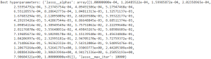
The ‘alphas’ parameter is an array of 50 values ranging from 10^-4 to 10^-1, evenly spaced on a log scale. These are the values of ‘alphas’ that were tried during the grid search process. The ‘max_iter’ parameter is set to 10000, which is the maximum iterations for the convergence to happen
6. Optimal Lambda:
The output shows the optimal value of lambda (also known as alpha) found by ‘LassoCV’. This is the value of alpha that resulted in the best cross-validation score.
Output:
Optimal Lambda: 0.0021209508879201904
The optimal lambda value is approximately 0.0021. This is the value of alpha that minimizes the cross-validation error value. And it is the value that the model will use for the alpha parameter.
7. Model performance:
Output:
Train MSE: 19.407125858891447

Test MSE: 11.349585984593896

Train R-squared: 0.7145150324137828

Test R-squared: 0.7527601793319424
- Mean squared Error (MSE): The MSE for the training set is 19.41 (approx) and for the test set is 11.37 (approx). MSE measures the average of the squares of the errors, that is, the average squared difference of the estimated values and the actual value. A lower MSE indicates that the model fits nicely with the data. So, the model has a lower MSE on the test set than on the training, which is a good sign normally because it suggests that the model is generalizing well to unseen data.
- R-squared: The R-squared value for the training set is 0.71 (approx) and for the test set is 0.75(approx). R-squared shows how well the model predicts the outcome of a dependent variable. An R-squared value of 100 percent indicates that the changes in the independent variables completely explain all changes in the dependent variable. So for the train R-squared, this means that 71% of the data was trained on. It is a good fit for the training data. For Test R-Squared, it means that the model can explain 75% of new, unseen data. It works well on data it hasn’t seen before. Since the test R-squared is a bit higher than the train R-squared, it means the model is performing well and isn’t just memorizing the training data. It is good at making predictions on new data too.
8. Visualizing the model performance:
To understand the performance of our lasso regression model better, we can visualize the actual versus predicted values using a plot. In this scatter plot, the x-axis represents the actual values, the y-axis represents the predicted values, and each point represents one of the instances in our dataset. The blue points are for the training data and the red are for the test data. The gray line represents an accurate prediction where the actual values equal the predicted values.
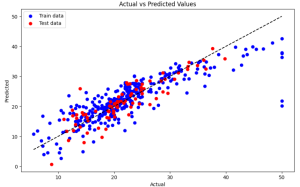
From the scatter plot, we can see that our model is doing a good job to some extent, of predicting the target variable, as most points are relatively close to the line, However, some points are scattered away from the grey line, indicating that there are some points where the model’s predictions are not well. This gives us a visual understanding of where our model is performing well and making errors.
Dataset for the above model: Housing Data