The Bias-Variance Tradeoff in Machine Learning

Understanding the bias-variance tradeoff in machine learning plays a crucial role in gaining knowledge about the performance of supervised learning algorithms. In this Blogspot, we will discuss the subtle balance that must be maintained between the model’s ability to capture the underlying patterns in the data (bias) and its capacity to generalize well to unseen data (variance).

Understanding Bias and Variance

Bias

Bias refers to the error arising from the assumptions or the learning made by the model. That means that models make certain assumptions or learn about the data and the underlying relationships to make the problem more understandable. These assumptions or the learning can introduce “Bias” into the model, causing it to miss or oversimplify the important patterns in the data. So basically, the higher the bias, the lesser the capturing of the underlying patterns, known as underfitting. Conversely, the lesser the bias, the more the model captures the underlying patterns and overcomes the underfitting.

Here are a few examples of assumptions  that can lead to bias

1. Linear Assumptions: Many models assume that the relationship between the input features and the target variable is directly proportional or linear, However, the relationships can be non-linear in real-world scenarios, and linear models may not be able to capture all the important underlying patterns.
2. Feature Independence: Some models assume that the input features are independent of each other, which is not the case in real-world datasets. This assumption can lead to inaccurate predictions when there are strong correlations or dependencies between features.
3. Feature selection: Selecting a certain type of feature to include in the model can also introduce bias. If important features are left out or irrelevant features are included, the model’s ability to capture the hidden patterns will not be accurate.

Bias plot of a model

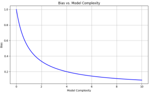
Inference:

• This plot shows how the bias decreases as the model complexity increases.
• At low model complexity values (left side of the plot), the bias is high, indicating that the model is too simple and cannot capture the underlying patterns in the data well, leading to underfitting.
• As the model complexity increases (moving right on the x-axis), the bias decreases because the model becomes more flexible and can better fit the data by capturing the underlying patterns.
• However, as the model complexity continues to increase further, the variance starts to increase, leading to potential overfitting issues.

Variance

Variance measures a model’s sensitivity to deviations or noise in the training data, which can come from sources like measurement errors, outliers (data points highly varying from the overall or original pattern), or irrelevant features. High variance models tend to overfit, capturing both underlying patterns and noise, which leads to poor generalization of new data. This is because the noise present in the training data may represent the true patterns. Conversely, low-variance models are more robust, and capture more stable patterns without being overly influenced by noise. They generalize better to unseen data by focusing on the true underlying patterns. Therefore, variance impacts the model’s ability to generalize effectively, with high variance indicating overfitting and low variance indicating better robustness to noise and fluctuations in the training data.

Variance plot of a model

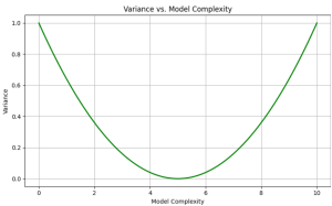
Inference:

• This plot shows how the variance increases as the model complexity increases, particularly after a certain plot.
• At low model complexity values (left side of the plot), the variance is low because the model is simple and cannot overfit the data.
• As the model complexity increases (moving right on the x-axis), the variance remains relatively low until a certain point (in this case, around model complexity=5).
• After this point, the variance increases rapidly, indicating that the model is becoming too complex and sensitive to noise or random fluctuations in the training data, potentially leading to overfitting.
• The trade-off tells us that the model complexity decreases when the bias increases, and the model becomes too simple or inefficient to capture the underlying important patterns.

The Tradeoff

The bias-variance tradeoff arises from a fundamental tension or conflict between two sources of error in machine learning: bias and variance. Reducing the bias often requires increasing model complexity, which in turn increases variance. Conversely, reducing variance often requires simplifying the model, which can increase bias. These errors impact model performance in different ways. Reducing one type of error often leads to an increase in the other, which is why we call it a tradeoff. So finding the right balance between the two sources of error is a much-needed step to take.

To illustrate:

1. Simple models (eg, linear regression): These models tend to have high bias, they may oversimplify complex data patterns. They often have low variance, they are less likely to be overly influenced by noise in the training data.
2. Complex models (eg, neural networks): These models have low bias, as they can potentially capture complex data patterns. They also have a high tendency to high variance as they are more sensitive to overfitting, getting influenced by noise, and random fluctuations in the training data.

This tradeoff exactly says that as you adjust your model’s complexity, you are importantly trying to attain a balance between bias and variance. The goal is to find the optimal point where the combined error from both sources is minimized, leading to a model that generalizes well to new, unseen data.

Bias-variance plot of a model

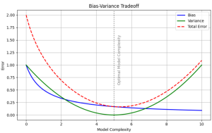
Inference:

• This plot combines the bias and variance curves, along with the total error curve (bias+variance).
• The total error curve exhibits the characteristic U-shaped pattern, with high error at both low and high model complexities.
• At low model complexity (left side of the plot), the bias is high, leading to underfitting and high total error.
• As the model complexity increases, the bias decreases, and the total error decreases initially.
• However, as the model complexity continues to increase further, the variance starts to increase rapidly, and the total error begins to rise again due to overfitting.
• The vertical dashed line represents the optimal model complexity, where the total error is minimized, and the bias-variance tradeoff of balanced.
• At this optimal point, the model is complex enough to capture the underlying patterns (low bias) but not too complex to overfit the noise (low variance).

Achieving the Right Balance

The goal of machine learning is to balance bias and variance, ensuring the model captures data patterns (low bias) without overfitting noise (low variance). This balance is achieved through various techniques such as:

1. Model selection: Choosing the right model complexity is crucial. Simple models line linear regression or decision trees have high bias but low variance, while complex models like neural networks have low bias and high variance. The goal is to match the model complexity to the problem and dataset, For example, neural networks are suitable for complex, non-linear problems with large datasets, while linear models suffice for simpler, linear separable problems.
2. Regularization: Techniques like L1(lasso) and L2(ridge) regularization for linear models, dropout and weight decay for neural networks, and pruning for decision trees add penalties for complexity. These methods encourage the model to find simpler solutions that generalize to unseen data,  reducing variance and preventing overfitting.
3. Cross-Validation: This technique involves splitting data into subsets (eg, k-fold cross-validation). The model is trained on one subset and evaluated on the other. Repeating this process multiple times and averaging the performance metrics helps assess the model’s generalization capabilities and tune hyperparameters (ed, regularization strength, model complexity) to achieve the best bias-variance balance.
4. Ensemble Methods: Combining multiple models with different biases and variances can create more robust predictions. Ensembles leverage the strengths of each model while mitigating their weaknesses. This often results in better generalization performance than individual models, as the combination can help reduce both bias and variance.

These techniques can be used together to achieve the desired bias-variance balance. For example, cross-validation can be used to select the respective model complexity (which affects the bias), perform regularization during training (which affects the variance), and combine different regularized models for improved model performance.

Conclusion

The bias-variance tradeoff is an important aspect of machine learning that tells us the need to maintain a good balance between two crucial aspects of model performance: pattern recognition and generalization (through learning). A solid understanding of the bias-variance tradeoff helps machine learning experts to develop models that not only perform well on training data but also maintain their accuracy and perform well when faced with new, unseen information. This leads to more accurate and reliable machine-learning solutions across various applications.

Also Read: L1 and L2 regularization