American Sign Language Recognition in Python using Deep Learning

By Rahul Makwana

In This Tutorial, we will be going to figure out how to apply transfer learning models vgg16 and resnet50 to perceive communication via gestures.

American Sign Language recognition (ASL)

 

here, we will learn how to apply the pre-trained model on the dataset using Python in Transfer Learning.

Dataset Link:- https://coderspacket.com/uploads/user_files/2020-08/American%20Sign%20Language%20recognition%20Dataset.rar

Some of the major problems faced by a person who is unable to speak are they cannot express their emotion as freely in this world. Utilize voice recognition and voice search systems in the smartphone(s). Audio results cannot be retrieved. They are not able to utilize (Artificial Intelligence/personal Butler) like google assistance, or Apple's SIRI, etc because all those apps are based on voice control.There is a need for such platforms for such kind of people. American Sign Language (ASL) is a complete, complex language that employs signs made by moving the hands combined with facial expressions and postures of the body. It is the go-to language of many North Americans who are not able to talk and is one of the various communication alternatives used by people who are deaf or hard-of-hearing.While sign language is very essential for deaf-mute people, to communicate both with normal people and with themselves, is still getting less attention from normal people. The importance of sign language has been tending to ignored unless there are areas of concern with individuals who are deaf-mute. One of the solutions to talk with the deaf-mute people is by using the mechanisms of sign language.The hand gesture is one of the methods used in sign language for non-verbal communication. It is most commonly used by deaf & dumb people who have hearing or talking disorders to communicate among themselves or with normal people. Various sign language systems have been developed by many manufacturers around the world but they are neither flexible nor cost-effective for the end-users.

 

There are various types of  transfer learning model for image classification such as 

1) Xception

2) VGG16

3) VGG19

4) ResNet50

5) InceptionV3

6) InceptionResnet

7) MobileNet

8) DenseNet

9) NASNet

10) MobileNetV2

 

Here, We are going to use VGG16 and RESNET50 to train the model. which are the pre-trained model.

 

What is the Pre-trained Model?

A pre-trained model has been previously trained on a dataset and contains the weights and biases that represent the features of whichever dataset it was trained on. Learned features are often transferable to different data. For example, a model trained on a large dataset of bird images will contain learned features like edges or horizontal lines that you would be transferable to your dataset.

 

Why use a Pre-trained Model?

 

Pre-trained models are beneficial to us for many reasons. By using a pre-trained model you are saving time. Someone else has already spent the time and compute resources to learn a lot of features and your model will get benefit from these pre-trained weights.

 

DATASET OVERVIEW:-

STEP-1:- Import Libraries and datasets

# Importing the Keras libraries and packages
from keras.applications.vgg16 import VGG16
from keras.applications.resnet50 import ResNet50
from keras.applications.vgg19 import VGG19
from keras.models import Model
from keras.preprocessing import image
from tensorflow.keras.layers import Input, Lambda ,Dense ,Flatten ,Dropout
import numpy as np
import tensorflow as tf
import matplotlib.pyplot as plt
%matplotlib inline
import os
import cv2
train_dir = "/kaggle/input/american-sign-language-recognition/training_set"
eval_dir = "/kaggle/input/american-sign-language-recognition/test_set"

 

STEP-2: Loading the data

#Helper function to load images from given directories
import keras
def load_images(directory):
    images = []
    labels = []
    for idx, label in enumerate(uniq_labels):
        for file in os.listdir(directory + "/" + label):
            filepath = directory + "/" + label + "/" + file
            image = cv2.resize(cv2.imread(filepath), (64, 64))
            images.append(image)
            labels.append(idx)
    images = np.array(images)
    labels = np.array(labels)
    return(images, labels)

uniq_labels = sorted(os.listdir(train_dir))
images, labels = load_images(directory = train_dir)

if uniq_labels == sorted(os.listdir(eval_dir)):
    X_eval, y_eval = load_images(directory = eval_dir)

Note: In the train-test split I have used the stratify argument on the labels. This argument ensures that the data is split evenly along all labels

now its time to apply sklearn's train test split to split the data here in our dataset there are two folders training set and test set in which here we are going to split X_train, X_test, y_train, y_test from the only training set and then we will predict the model on an unseen dataset.

from sklearn.model_selection import train_test_split
X_train, X_test, y_train, y_test = train_test_split(images, labels, test_size = 0.2, stratify = labels)

n = len(uniq_labels)
train_n = len(X_train)
test_n = len(X_test)

print("Total number of symbols: ", n)
print("Number of training images: " , train_n)
print("Number of testing images: ", test_n)

eval_n = len(X_eval)
print("Number of evaluation images: ", eval_n)

STEP-3:Preprocessing: One-hot encoding the data

This conversion will turn the one-dimensional array of labels into a two-dimensional array. Each row in the two-dimensional array of one-hot encoded labels corresponds to a different label.

 

as you can see in the below picture first column indicates the column second is indicating label encoding which we can do by label encoding and the last column is one hot encoding. in which whenever the A occurs it will give an output of 1 otherwise 0 same as when B is encountered it will give an output of 1 in 2nd-row 2nd column and so on.

 

For instance,

 

0 is encoded as [1, 0, 0],

1 is encoded as [0, 1, 0], and

2 is encoded as [0, 0, 1].

y_train = keras.utils.to_categorical(y_train)
y_test = keras.utils.to_categorical(y_test)
y_eval = keras.utils.to_categorical(y_eval)

now just checking that is it converted or not.

print(y_train[0])
print(len(y_train[0]))

OUTPUT:-

[0. 0. 0. 0. 0. 0. 0. 0. 0. 0. 0. 0. 0. 0. 0. 0. 0. 0. 0. 0. 0. 0. 0. 0.

1. 0. 0. 0. 0. 0. 0. 0. 0. 0. 0. 1. 0. 0. 0. 0.]

40

 

We see that we have successfully one-hot encoded the labels. The length is 40, to make room for the 40 labels A to Space in our data.

STEP-5: Preprocessing - Normalize RGB values

 

Normalization will help us remove distortions caused by lights and shadows in an image.Now let us look at how the image data is stored. There are three components for each image - one component each for the Red, Green, and Blue (RGB) channels. The component values are stored as integer numbers in the range 0 to 255.If, however, we divide by 255 the range can be described with a 0.0-1.0 where 0.0 means 0 (0x00 in hex) and 1.0 means 255 (0xFF in hex).

 

X_train = X_train.astype('float32')/255.0
X_test = X_test.astype('float32')/255.0
X_eval = X_eval.astype('float32')/255.0

 

Now its time to apply our models:-

 

NOTE:-as you can see in the below image for the transfer learning model we have to cut the last fully connected layer because we have to add our own fully connected layer. Now we have 40 classes so we will add a fully connected layer of 40 classes.This pre-trained model has already been trained by someone so we do not have to again train the model we just have to add our fully connected layers and just merge them with the pre-trained model and then train our last fully connected layer which we are adding. 

 

initializing all the models

 

VGG16:-

VGG16 is a convolution neural net (CNN ) architecture which was used to win ILSVR(Imagenet) competition in 2014. It is considered to be one of the excellent vision model architecture till date. Most unique thing about VGG16 is that instead of having a large number of hyper-parameter they focused on having convolution layers of 3x3 filter with a stride 1 and always used same padding and maxpool layer of 2x2 filter of stride 2. It follows this arrangement of convolution and max pool layers consistently throughout the whole architecture. In the end it has 2 FC(fully connected layers) followed by a softmax for output. The 16 in VGG16 refers to it has 16 layers that have weights. This network is a pretty large network and it has about 138 million (approx) parameters.

 

The architecture of VGG16:-

 

 

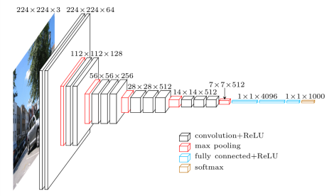
#Initialising vgg16 
classifier_vgg16 = VGG16(input_shape= (64,64,3),include_top=False,weights='imagenet')

OUTPUT:-

 

Downloading data from https://storage.googleapis.com/tensorflow/keras-applications/vgg16/vgg16_weights_tf_dim_ordering_tf_kernels_notop.h5

58892288/58889256 [==============================] - 0s 0us/step

 

Architecture of RESNET50:-

#Initialising resnet50 
classifier_resnet = ResNet50(input_shape=(64,64,3),include_top=False,weights='imagenet')

OUTPUT:-

 

Downloading data from https://storage.googleapis.com/tensorflow/keras-applications/resnet/resnet50_weights_tf_dim_ordering_tf_kernels_notop

.h5

94773248/94765736 [==============================] - 2s 0us/step

 

#don't train existing weights for vgg16
for layer in classifier_vgg16.layers:
    layer.trainable = False

#don't train existing weights for resnet50
for layer in classifier_resnet.layers:
    layer.trainable = False

Compiling the Model:-

#VGG16
classifier1 = classifier_vgg16.output#head mode
classifier1 = Flatten()(classifier1)#adding layer of flatten
classifier1 = Dense(units=256, activation='relu')(classifier1)
classifier1 = Dropout(0.6)(classifier1)
classifier1 = Dense(units=40, activation='softmax')(classifier1)

model = Model(inputs = classifier_vgg16.input , outputs = classifier1)
model.compile(optimizer='adam', loss='categorical_crossentropy', metrics=['accuracy'])

#resnet50
classifier2 = classifier_resnet.output#head mode
classifier2 = Flatten()(classifier2)#adding layer of flatten
classifier2 = Dropout(0.6)(classifier2)
classifier2 = Dense(units=40, activation='softmax')(classifier2)

model2 = Model(inputs = classifier_resnet.input , outputs = classifier2)
model2.compile(optimizer='adam', loss='categorical_crossentropy', metrics=['accuracy'])

#summary of vgg16
model.summary()

#summary of resnet50
model2.summary()

its time to train our both model vgg16 and resnet50

VGG16:-

#fit the model
#it will take some time to train
#vgg16
history = model.fit(X_train, y_train, epochs =5, batch_size = 32,validation_data=(X_test,y_test))

OUTPUT:-

 

Epoch 1/5

1509/1509 [==============================] - 24s 16ms/step - loss: 0.2013 - accuracy: 0.9561 - val_loss: 9.9571e-04 - val_accuracy: 1.0000

Epoch 2/5

1509/1509 [==============================] - 23s 15ms/step - loss: 0.0111 - accuracy: 0.9985 - val_loss: 3.6338e-04 - val_accuracy: 1.0000

Epoch 3/5

1509/1509 [==============================] - 23s 15ms/step - loss: 0.0131 - accuracy: 0.9966 - val_loss: 5.9608e-05 - val_accuracy: 1.0000

Epoch 4/5

1509/1509 [==============================] - 23s 15ms/step - loss: 0.0108 - accuracy: 0.9969 - val_loss: 2.0817e-05 - val_accuracy: 1.0000

Epoch 5/5

1509/1509 [==============================] - 23s 15ms/step - loss: 0.0111 - accuracy: 0.9964 - val_loss: 2.1358e-05 - val_accuracy: 1.0000

 

ResNet50:-

#fit the model
#resnet50
history2 = model2.fit(X_train, y_train, epochs =5, batch_size = 32,validation_data=(X_test,y_test))

OUTPUT:-

 

Epoch 1/5

1509/1509 [==============================] - 30s 20ms/step - loss: 0.3123 - accuracy: 0.9387 - val_loss: 0.0260 - val_accuracy: 0.9988

Epoch 2/5

1509/1509 [==============================] - 28s 19ms/step - loss: 0.0576 - accuracy: 0.9880 - val_loss: 0.0102 - val_accuracy: 0.9989

Epoch 3/5

1509/1509 [==============================] - 29s 19ms/step - loss: 0.0363 - accuracy: 0.9911 - val_loss: 0.0055 - val_accuracy: 0.9994

Epoch 4/5

1509/1509 [==============================] - 29s 19ms/step - loss: 0.0287 - accuracy: 0.9930 - val_loss: 0.0049 - val_accuracy: 0.9993

Epoch 5/5

1509/1509 [==============================] - 28s 19ms/step - loss: 0.0266 - accuracy: 0.9924 - val_loss: 0.0016 - val_accuracy: 0.9999

 

Saving the model:-

 

# Saving the model of vgg16
model.save('model_vgg16.h5')
# Saving the model of resnet
model2.save('model_resnet.h5')

Accuracy of VGG16:-

score = model.evaluate(x = X_test, y = y_test, verbose = 0)
print('Accuracy for test images:', round(score[1]*100, 3), '%')
score = model.evaluate(x = X_eval, y = y_eval, verbose = 0)
print('Accuracy for evaluation images:', round(score[1]*100, 3), '%')

OUTPUT:-

 

Accuracy for test images: 99.0 %

Accuracy for evaluation images: 99.0 %

 

Accuracy of RESNET50:-

score = model2.evaluate(x = X_test, y = y_test, verbose = 0)
print('Accuracy for test images:', round(score[1]*100, 3), '%')
score = model2.evaluate(x = X_eval, y = y_eval, verbose = 0)
print('Accuracy for evaluation images:', round(score[1]*100, 3), '%')

OUTPUT:-

 

Accuracy for test images: 99.992 %

Accuracy for evaluation images: 99.0 %

 

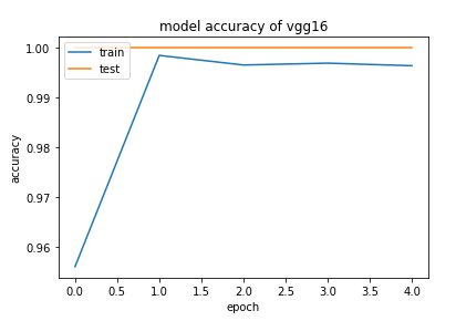
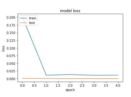
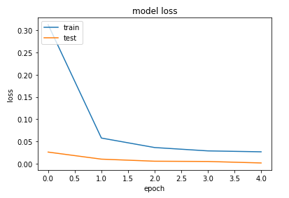
VGG16 accuracy and loss plot:-

#vgg16
# summarize history for accuracy
import matplotlib.pyplot as plt
plt.plot(history.history['accuracy'])
plt.plot(history.history['val_accuracy'])
plt.title('model accuracy of vgg16')
plt.ylabel('accuracy')
plt.xlabel('epoch')
plt.legend(['train', 'test'], loc='upper left')
plt.show()

# summarize history for loss
plt.plot(history.history['loss'])
plt.plot(history.history['val_loss'])
plt.title('model loss')
plt.ylabel('loss')
plt.xlabel('epoch')
plt.legend(['train', 'test'], loc='upper left')
plt.show()

                                               

 

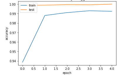
resnet50 accuracy and loss plot:-

#resnet50
# summarize history for accuracy
import matplotlib.pyplot as plt
plt.plot(history2.history['accuracy'])
plt.plot(history2.history['val_accuracy'])
plt.title('model accuracy of resnet50')
plt.ylabel('accuracy')
plt.xlabel('epoch')
plt.legend(['train', 'test'], loc='upper left')
plt.show()

# summarize history for loss
plt.plot(history2.history['loss'])
plt.plot(history2.history['val_loss'])
plt.title('model loss')
plt.ylabel('loss')
plt.xlabel('epoch')
plt.legend(['train', 'test'], loc='upper left')
plt.show()

                                           

VGG16 confusion matrix:-

 

A confusion matrix is a table that is often used to describe the performance of a classification model (or "classifier") on a set of test data for which the true values are known. Each row of the matrix represents the instances in an actual class while each column represents the instances in an predicted class (or vice versa).

 

The name stems from the fact that it makes it easy to see if the system is confusing two classes (i.e. commonly mislabeling one as another).

 

I will plot confusion matrices for both the testing and evaluation data. Since I have to go through the same code twice, it makes sense to first define a function that helps us plot these matrices. The function below does exactly that. The code y = np.argmax(y, axis = 1) converts the 2D array y into a 1D array with number labels for each image.

 

I do this for both the true and the predicted values. Additionally, plotting the confusion matrix with a cmap automatically fills it with a colour gradient showing how many of the values were correctly predicted. The for loop at the end of the function fills each cell of the matrix with the number of predictions that correspond to that cell.

 

Note that our the matrix is not normalized, and the total number of testing images per label were 300.

 

#Helper function to plot confusion matrix
from sklearn.metrics import confusion_matrix
import itertools
def plot_confusion_matrix(y, y_pred):
    y = np.argmax(y, axis = 1)
    y_pred = np.argmax(y_pred, axis = 1)
    cm = confusion_matrix(y, y_pred)
    plt.figure(figsize = (24, 20))
    ax = plt.subplot()
    plt.imshow(cm, interpolation = 'nearest', cmap = plt.cm.Purples)
    plt.colorbar()
    plt.title("Confusion Matrix")
    tick_marks = np.arange(len(uniq_labels))
    plt.xticks(tick_marks, uniq_labels, rotation=45)
    plt.yticks(tick_marks, uniq_labels)
    plt.ylabel('True label')
    plt.xlabel('Predicted label')
    ax.title.set_fontsize(20)
    ax.xaxis.label.set_fontsize(16)
    ax.yaxis.label.set_fontsize(16)
    limit = cm.max() / 2.
    for i, j in itertools.product(range(cm.shape[0]), range(cm.shape[1])):
        plt.text(j, i, format(cm[i, j], 'd'), horizontalalignment = "center",color = "white" if cm[i, j] > limit else "black")
    plt.show()
y_test_pred = model.predict(X_test, batch_size = 64, verbose = 0)
plot_confusion_matrix(y_test, y_test_pred)

 

RESNET50 confusion matrix:-

y_test_pred = model2.predict(X_test, batch_size = 64, verbose = 0)
plot_confusion_matrix(y_test, y_test_pred)

 

Predictions:-

# for only one prediction
import numpy as np
from keras.preprocessing import image
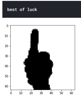
test_image = image.load_img('/kaggle/input/american-sign-language-recognition/test_set/best of luck/11.png',target_size=(64,64))
plt.imshow(test_image)
test_image = image.img_to_array(test_image)
test_image = np.expand_dims(test_image, axis=0)
result = model.predict(test_image)

if result[0][0] == 1:             
    prediction = '1'
elif result[0][1] == 1:
    prediction = '10'
elif result[0][2] == 1:
    prediction = '2'
elif result[0][3] == 1:
    prediction = '3'
elif result[0][4] == 1:
    prediction = '4'
elif result[0][5] == 1:
    prediction = '5'
elif result[0][6] == 1:
    prediction = '6'
elif result[0][7] == 1:
    prediction = '7'
elif result[0][8] == 1:
    prediction = '8'
elif result[0][9] == 1:
    prediction = '9'
elif result[0][10] == 1:
    prediction = 'A'
elif result[0][11] == 1:
    prediction = 'B'
elif result[0][12] == 1:
    prediction = 'C'
elif result[0][13] == 1:
    prediction = 'D'
elif result[0][14] == 1:
    prediction = 'E'
elif result[0][15] == 1:
    prediction = 'F'
elif result[0][16] == 1:
    prediction = 'G'
elif result[0][17] == 1:
    prediction = 'H'
elif result[0][18] == 1:
    prediction = 'I'
elif result[0][19] == 1:
    prediction = 'J'
elif result[0][20] == 1:
    prediction = 'K'
elif result[0][21] == 1:
    prediction = 'L'
elif result[0][22] == 1:
    prediction = 'M'
elif result[0][23] == 1:
    prediction = 'N'
elif result[0][24] == 1:
    prediction = 'O'
elif result[0][25] == 1:
    prediction = 'P'
elif result[0][26] == 1:
    prediction = 'Q'
elif result[0][27] == 1:
    prediction = 'R'
elif result[0][28] == 1:
    prediction = 'S'
elif result[0][29] == 1:
    prediction = 'T'
elif result[0][30] == 1:
    prediction = 'U'
elif result[0][31] == 1:
    prediction = 'V'
elif result[0][32] == 1:
    prediction = 'W'
elif result[0][33] == 1:
    prediction = 'X'
elif result[0][34] == 1:
    prediction = 'Y'
elif result[0][35] == 1:
    prediction = 'Z'
elif result[0][36] == 1:
    prediction = 'best of luck'
elif result[0][37] == 1:
    prediction = 'fuck you'
elif result[0][38] == 1:
    prediction = 'i love you'
else:
    prediction = '  '
    
print(prediction)

OUTPUT:-

our output will look like this and it is just one prediction.

conclusion:- in this tutorial we learned how to apply vgg16 and resnet50 transfer learning models to predict the sign language using hand gestures.