Covid-19 chest x-ray detection using Python in Deep Learning
 Rahul Makwana
Aug 08, 2020
Rahul Makwana
Aug 08, 2020
In this Tutorial, we will apply a convolutional neural network using Python in Deep Learning and also do prediction.
Covid-19 chest x-ray detection
The novel coronavirus 2019 (COVID-2019), which first appeared in Wuhan city of China in December 2019, spread rapidly around the world and became a pandemic. It has caused a devastating effect on both daily lives, public health, and the global economy. It is critical to detect the positive cases as early as possible so as to prevent the further spread of this epidemic and to quickly treat affected patients. Our CNN model produced a classification accuracy of 94.00% on validation data.
Dataset link:- https://drive.google.com/file/d/1i-dS_NqHSKPGMf9jH8fU725Ljv_42zvs/view?usp=sharing
here, we have 3 folders in which two of them are used for training and testing and another one is a mix image dataset where all the COVID and normal patients x-rays are a mix.
What is CNN?
In deep learning, a convolutional neural network is a class of deep neural networks, most commonly applied to analyzing visual imagery. Convolutional networks were inspired by biological processes in that the connectivity pattern between neurons resembles the organization of the animal visual cortex.
Architecture of CNN:-
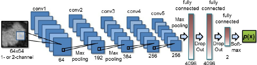 Building CNN
In order to build CNN, we need to import a couple of modules from KERAS:
1. Sequential for initializing the neural network
2. Dense for adding a densely connected neural network layer
3. Convolutio2D for adding the convolutional neural network layer
4. ReLU stands for the Rectified Linear Unit for a non-linear operation. The output is ƒ(x) = max(0,x).
5. The pooling Layer Pooling layers section would reduce the number of parameters when the images are too large. Spatial pooling also called subsampling or downsampling which reduces the dimensionality of each map but retains important information.
We have used max-pooling function Max pooling takes the largest element from the rectified feature map. Taking the largest element could also take the average pooling. Sum of all elements in the feature map call as sum pooling.
6. Flattening is converting the data into a 1-dimensional array for inputting it to the next layer. We flatten the output of the convolutional layers to create a single long feature vector. And it is connected to the final classification model, which is called a fully-connected layer.
STEP:1 importing libraries for CNN
import tensorflow as tf
import numpy as np
from tensorflow.keras.preprocessing.image import ImageDataGenerator
import matplotlib.pyplot as plt
from keras.preprocessing import image
import os
from sklearn.metrics import confusion_matrix ,classification_report
import seaborn as sns
STEP:2- Making simple CNN model
# Initialising the CNN
classifier = tf.keras.models.Sequential()

classifier.add(tf.keras.layers.Convolution2D(filters=32, kernel_size=3, padding="same", input_shape=(224, 224, 3),
                                             activation='relu'))

classifier.add(tf.keras.layers.MaxPooling2D(pool_size=2, strides=2, padding='valid'))

classifier.add(tf.keras.layers.Convolution2D(filters=64, kernel_size=3, padding="same", activation="relu"))
classifier.add(tf.keras.layers.MaxPooling2D(pool_size=2, strides=2, padding='valid'))


classifier.add(tf.keras.layers.Convolution2D(filters=64, kernel_size=3, padding="same", activation="relu"))
classifier.add(tf.keras.layers.Dropout(0.2))
classifier.add(tf.keras.layers.MaxPooling2D(pool_size=2, strides=2, padding='valid'))


classifier.add(tf.keras.layers.Convolution2D(filters=128, kernel_size=3, padding="same", activation="relu"))
classifier.add(tf.keras.layers.Dropout(0.2))
classifier.add(tf.keras.layers.MaxPooling2D(pool_size=2, strides=2, padding='valid'))

classifier.add(tf.keras.layers.Convolution2D(filters=256, kernel_size=3, padding="same", activation="relu"))
classifier.add(tf.keras.layers.Dropout(0.2))
classifier.add(tf.keras.layers.MaxPooling2D(pool_size=2, strides=2, padding='valid'))

classifier.add(tf.keras.layers.Convolution2D(filters=64, kernel_size=3, padding="same", activation="relu"))
classifier.add(tf.keras.layers.MaxPooling2D(pool_size=2, strides=2, padding='valid'))


classifier.add(tf.keras.layers.Flatten())

classifier.add(tf.keras.layers.Dense(units=128, activation='relu'))
classifier.add(tf.keras.layers.Dense(units=1, activation='sigmoid'))

classifier.compile(optimizer='adam', loss='binary_crossentropy', metrics=['accuracy'])
classifier.summary()
STEP:3 applying image data generator
train_datagen = ImageDataGenerator(rescale=1. / 255,
                                   shear_range=0.2,
                                   zoom_range=0.2,
                                   horizontal_flip=True)

test_datagen = ImageDataGenerator(rescale=1. / 255)

training_set = train_datagen.flow_from_directory('/kaggle/input/corona-chest-xray-prediction/Data/train',
                                                 target_size=(224,224),
                                                 batch_size=32,
                                                 class_mode='binary')

test_set = test_datagen.flow_from_directory('/kaggle/input/corona-chest-xray-prediction/Data/test',
                                            target_size=(224,224),
                                            batch_size=32,
                                            class_mode='binary')
OUTPUT:-
Found 100 images belonging to 2 classes.
Found 100 images belonging to 2 classes.

now its time to train our model.
history = classifier.fit(training_set,
                         steps_per_epoch=4,
                         epochs=25,
                         validation_data=test_set,
                         validation_steps=4)

classifier.save('my_model.h5')
OUTPUT:-
Epoch 1/25
4/4 [==============================] - 16s 4s/step - loss: 0.5497 - accuracy: 0.6300 - val_loss: 0.4475 - val_accuracy: 0.9400
Epoch 2/25
4/4 [==============================] - 14s 4s/step - loss: 0.5195 - accuracy: 0.7400 - val_loss: 0.4609 - val_accuracy: 0.8500
Epoch 3/25
4/4 [==============================] - 14s 4s/step - loss: 0.4992 - accuracy: 0.7100 - val_loss: 0.5447 - val_accuracy: 0.6600
Epoch 4/25
4/4 [==============================] - 17s 4s/step - loss: 0.5386 - accuracy: 0.8300 - val_loss: 0.4902 - val_accuracy: 0.9000
Epoch 5/25
4/4 [==============================] - 14s 4s/step - loss: 0.3055 - accuracy: 0.9100 - val_loss: 0.2659 - val_accuracy: 0.9000
Epoch 6/25
4/4 [==============================] - 15s 4s/step - loss: 0.2778 - accuracy: 0.8700 - val_loss: 0.1575 - val_accuracy: 0.9300
Epoch 7/25
4/4 [==============================] - 14s 3s/step - loss: 0.2214 - accuracy: 0.9300 - val_loss: 0.1680 - val_accuracy: 0.9400
Epoch 8/25
4/4 [==============================] - 14s 4s/step - loss: 0.2314 - accuracy: 0.9400 - val_loss: 0.2042 - val_accuracy: 0.9300
Epoch 9/25
4/4 [==============================] - 14s 4s/step - loss: 0.1460 - accuracy: 0.9400 - val_loss: 0.1375 - val_accuracy: 0.9500
Epoch 10/25
4/4 [==============================] - 15s 4s/step - loss: 0.1341 - accuracy: 0.9500 - val_loss: 0.1351 - val_accuracy: 0.9600
Epoch 11/25
4/4 [==============================] - 17s 4s/step - loss: 0.1840 - accuracy: 0.9400 - val_loss: 0.3678 - val_accuracy: 0.8300
Epoch 12/25
4/4 [==============================] - 16s 4s/step - loss: 0.1345 - accuracy: 0.9400 - val_loss: 0.1788 - val_accuracy: 0.9400
Epoch 13/25
4/4 [==============================] - 14s 3s/step - loss: 0.1632 - accuracy: 0.9500 - val_loss: 0.1443 - val_accuracy: 0.9600
Epoch 14/25
4/4 [==============================] - 15s 4s/step - loss: 0.1061 - accuracy: 0.9400 - val_loss: 0.1558 - val_accuracy: 0.9600
Epoch 15/25
4/4 [==============================] - 14s 4s/step - loss: 0.1362 - accuracy: 0.9500 - val_loss: 0.1876 - val_accuracy: 0.9600
Epoch 16/25
4/4 [==============================] - 14s 4s/step - loss: 0.0374 - accuracy: 0.9900 - val_loss: 0.2031 - val_accuracy: 0.9500
Epoch 17/25
4/4 [==============================] - 13s 3s/step - loss: 0.0938 - accuracy: 0.9700 - val_loss: 0.2446 - val_accuracy: 0.9300
Epoch 18/25
4/4 [==============================] - 15s 4s/step - loss: 0.0314 - accuracy: 0.9800 - val_loss: 0.1101 - val_accuracy: 0.9500
Epoch 19/25
4/4 [==============================] - 14s 4s/step - loss: 0.1027 - accuracy: 0.9700 - val_loss: 0.1028 - val_accuracy: 0.9700
Epoch 20/25
4/4 [==============================] - 15s 4s/step - loss: 0.0484 - accuracy: 0.9700 - val_loss: 0.1731 - val_accuracy: 0.9400
Epoch 21/25
4/4 [==============================] - 14s 4s/step - loss: 0.0454 - accuracy: 0.9900 - val_loss: 0.1259 - val_accuracy: 0.9700
Epoch 22/25
4/4 [==============================] - 15s 4s/step - loss: 0.2145 - accuracy: 0.9200 - val_loss: 0.4202 - val_accuracy: 0.8400
Epoch 23/25
4/4 [==============================] - 16s 4s/step - loss: 0.1126 - accuracy: 0.9500 - val_loss: 0.2662 - val_accuracy: 0.8900
Epoch 24/25
4/4 [==============================] - 15s 4s/step - loss: 0.0731 - accuracy: 0.9800 - val_loss: 0.3029 - val_accuracy: 0.9200
Epoch 25/25
4/4 [==============================] - 15s 4s/step - loss: 0.0591 - accuracy: 0.9800 - val_loss: 0.2380 - val_accuracy: 0.9400
evaluating on test set:-
# evaluation on test set
loaded_model = tf.keras.models.load_model('my_model.h5')
loaded_model.evaluate(test_set)
OUTPUT:-
as you can see above loss is 0.23 and accuracy is almost 94.00%
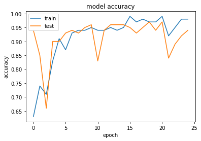
STEP:4 Plotting loss and accuracy
#plot accuracy and loss
import matplotlib.pyplot as plt
plt.plot(history.history['accuracy'])
plt.plot(history.history['val_accuracy'])
plt.title('model accuracy')
plt.ylabel('accuracy')
plt.xlabel('epoch')
plt.legend(['train', 'test'], loc='upper left')
plt.show()
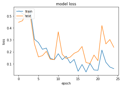
plt.plot(history.history['loss'])
plt.plot(history.history['val_loss'])
plt.title('model loss')
plt.ylabel('loss')
plt.xlabel('epoch')
plt.legend(['train', 'test'], loc='upper left')
plt.show()
STEP:5 confusion matrix
# plot confusion metrix
y_pred = []
y_test = []
import os

for i in os.listdir("../input/corona-chest-xray-prediction/Data/test/Normal"):
    img = image.load_img("../input/corona-chest-xray-prediction/Data/test/Normal/" + i, target_size=(224,224))
    img = image.img_to_array(img)
    img = np.expand_dims(img, axis=0)
    p = classifier.predict_classes(img)
    y_test.append(p[0, 0])
    y_pred.append(1)

for i in os.listdir("../input/corona-chest-xray-prediction/Data/test/Covid"):
    img = image.load_img("../input/corona-chest-xray-prediction/Data/test/Covid/" + i, target_size=(224,224))
    img = image.img_to_array(img)
    img = np.expand_dims(img, axis=0)
    p = classifier.predict_classes(img)
    y_test.append(p[0, 0])
    y_pred.append(0)

y_pred = np.array(y_pred)
y_test = np.array(y_test)

cm = confusion_matrix(y_pred, y_test)
sns.heatmap(cm, cmap="plasma", annot=True)

from sklearn.metrics import classification_report
print(classification_report(y_pred, y_test))
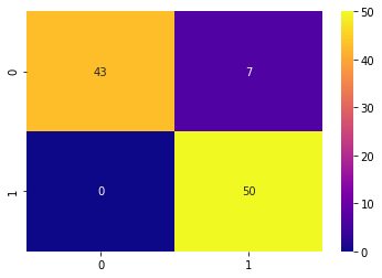
                                                 precision    recall  f1-score   support

                                            0       1.00      0.86      0.92        50
                                            1       0.88      1.00      0.93        50

                                     accuracy                           0.93       100
                                    macro avg       0.94      0.93      0.93       100
                                 weighted avg       0.94      0.93      0.93       100
STEP:6 Prediction
# for only one prediction
import numpy as np
from keras.preprocessing import image

test_image = image.load_img('/kaggle/input/Data/test/Covid/covid-19-pneumonia-28.png',target_size=(224,224))
plt.imshow(test_image)
test_image = image.img_to_array(test_image)
test_image = np.expand_dims(test_image, axis=0)
result = loaded_model.predict(test_image)
training_set.class_indices
if result[0][0] == 1:
    prediction = 'Normal'
else:
    prediction = 'Covid'
print(prediction)
OUTPUT:-
covid
# for only one prediction
import numpy as np
from keras.preprocessing import image

test_image = image.load_img('/kaggle/input/Data/original test set/NORMAL2-IM-0112-0001.jpeg',target_size=(224,224))
plt.imshow(test_image)
test_image = image.img_to_array(test_image)
test_image = np.expand_dims(test_image, axis=0)
result = loaded_model.predict(test_image)
training_set.class_indices
if result[0][0] == 1:
    prediction = 'Normal'
else:
    prediction = 'Covid'
print(prediction)
OUTPUT:-
Normal
conclusion:- in this tutorial, we learned what is the convolutional neural network and how to apply CNN on the small dataset and we gained 94% accuracy on test data.
Project Files
| .. | ||
| This directory is empty. | ||
