DeRem : Detection and Removal of Outliers for Univariate Variables

By Rohit Naresh Saktel

The project named - 'DeRem' - is all about the detection and removal of outliers from any univariate variable dataset.

The practical knowledge of the project can be easily gained with the help of a working example.

Therefore, the working example of the project is shown below and at the end, I will share the format of the source code for both kinds which can be easily accessible and understandable.

 

Detection and Removal of Outliers - For Normal Distribution :

Data can be "distributed" (spread out) in different ways.It can be spread out more on the left, or more on the right, or it can be all jumbled up.

But there are many cases where the data tends to be around a central value with no bias left or right, and it gets close to a "Normal Distribution".

The Normal Distribution has:

• mean = median = mode
• symmetry about the center
• 50% of values less than the mean
  and 50% greater than the mean

This can be observe at the time of visualization. The Blue curve in the plot denotes the Normal Distribution.

 

Some operations are needed before the steps for the detection and removal of outliers which are as follows :

 

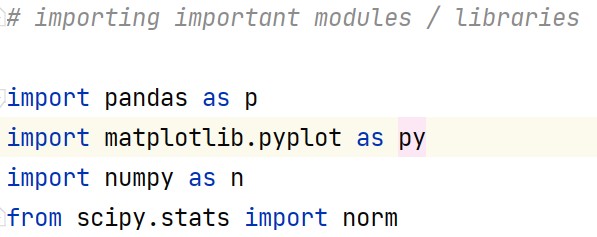
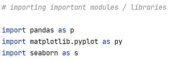
Operation 1 : Importing important modules / libraries -

Operation 2 : Reading UNIVARIATE VARIABLE dataset file in csv format -

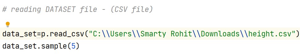
Output - 

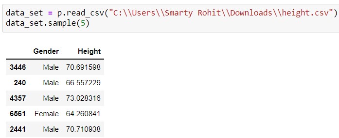
Note - The output section is captured form jupyter notebook.

Operation 3 : Visualization of data set (NORMAL DISTRIBUTION) -

In visualization, we have made use of a histogram plot, which can easily fulfill the condition for the normal distribution, mentioned above.

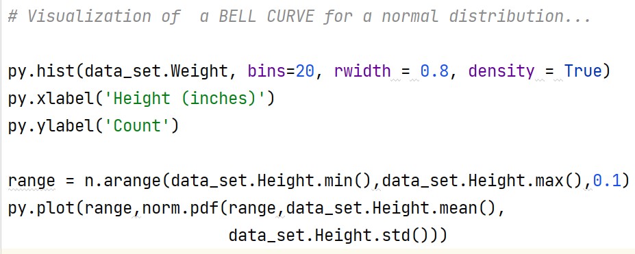
Output - 

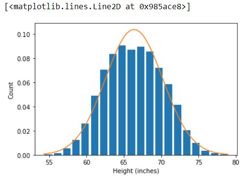
Here, you can observe a bell - curve, which is nothing but a normal distribution. Along with the conditions for normal distribution is somehow satisfied, as we can observe through the plot. Currently, the dataset involves some counts of outliers that divert those conditions. After cleansing the data, the plot will get changed.

 

Steps for Detection of Outliers ---> using z-score / standard score

For Normal Distribution,

The data points which fall below mean-3*(sigma) or above mean+3*(sigma) are outliers.

where mean and sigma are the average value and standard deviation of a particular column.

And, 

z-score is a way to achieve the same thing.

 

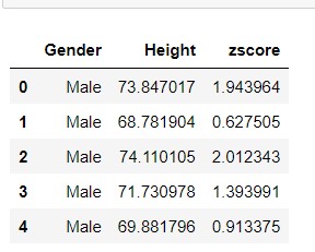
Step 1 : Computation of z-score

z-score = data_value (x) - mean / standard deviation (sigma)  ---------> Formula for calculation of z-score

 

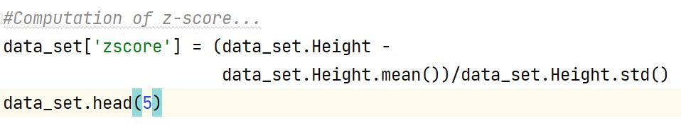
Output - 

 

 

Step 2 : Detection of Outliers

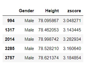
Here we will create a new dataframe (outlier_detect) that includes only the outliers as per the condition mentioned at the start.

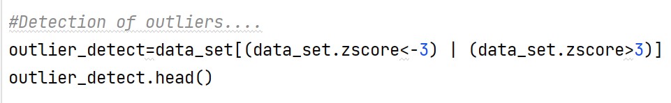
Output - 

The output contains values which are greater 3 and less than -3 as satisfied the condition of outliers for normal distribution. 

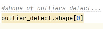
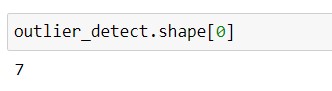
we can have look at shape of dataframe or numbers of outliers present in new dataframe as :

corresponding output - 

Step for Removal of Outliers ---> using z-score / standard score

This step involves the removal of a sub-data frame from the original data frame which thus results in the removal of all outliers from the dataset.

 

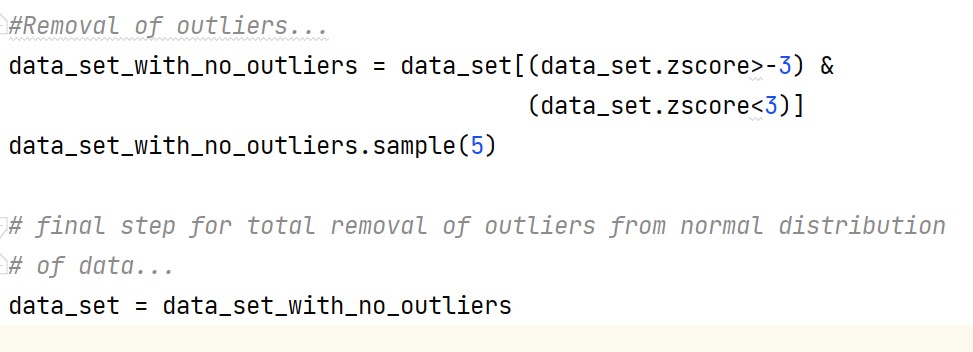
Output - 

 

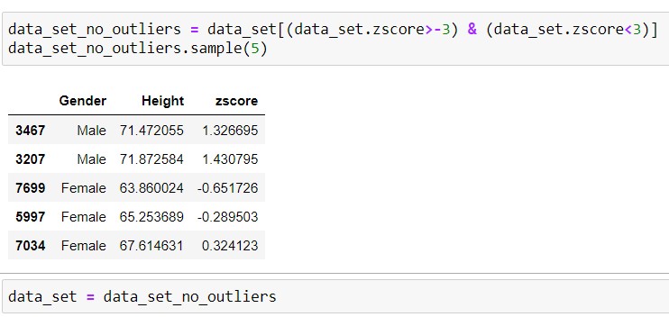
The drawn sample output clearly shows the data values with z-score (>-3 and <3) and excluding the remainings(i.e., outliers).

Hence, we have successfully detected and removed the outliers from the dataset.

 

This can be re-verified with the help of visualization of new dataset using histogram plot.

 

Visualization of a new dataset

Code - 

 

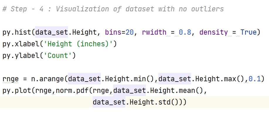
Output - 

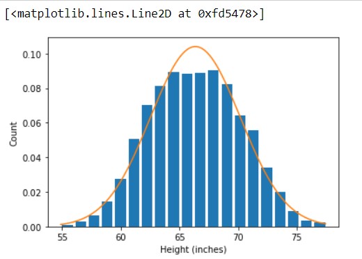
Thus, here is the final output. You can have a comparison between the two plots and can easily observe the changes that occur after and before consecutively.

 

Detection and Removal of Outliers - For Skewed Distribution :

Data can be "skewed", meaning it tends to have a long tail (data values scatter more) on one side or the other : Negative skew, No skew, Positive skew

Negative skew - long tail on the negative side of the peak or " skewed to the left "

No skew - A normal distribution

Positive skew - long tail on the positive side of the peak or " skewed to the right "

 

This can be observe at the time of visualization.

Some operations are needed before the steps for the detection and removal of outliers which are as follows : 

Operation 1 : Importing important modules / libraries -

 

Operation 2 : Reading UNIVARIATE VARIABLE dataset file in csv format -

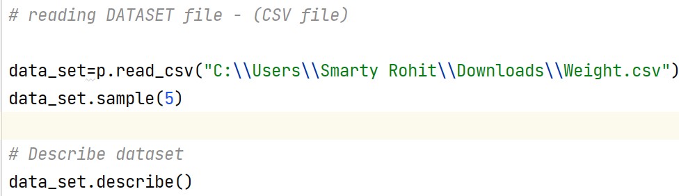
Output - 

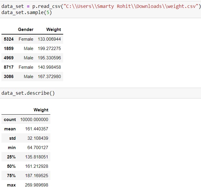
Note - The output section is captured form jupyter notebook.

 

Operation 3 : Visualization of data set (SKEWED DISTRIBUTION) -

In visualization for the skewed distribution of data, we have make use of Boxplot plot .

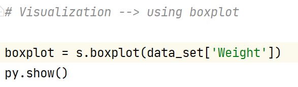
Output - 

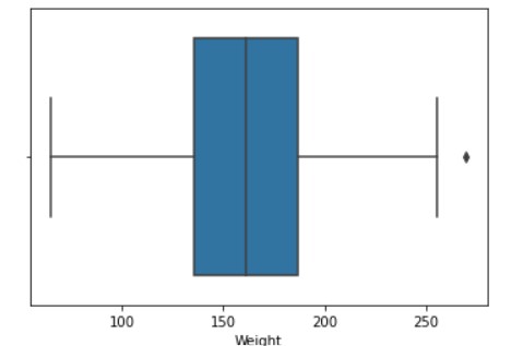
We can clearly observe the outlier shown / plot in the dataset.

 

Steps for Detection of Outliers ---> using Interqaurtile Range / IQR

For skewed distribution,

The data points which fall below Q1 – 1.5 IQR or above Q3 + 1.5 IQR are outliers.

where Q1 and Q3 are the 25th and 75th percentile of the dataset respectively, and IQR represents the inter-quartile range and given by Q3 – Q1.

 

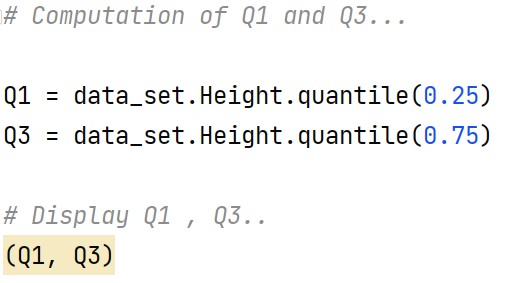
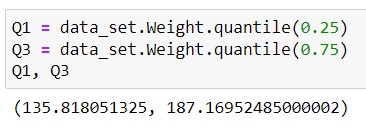
Step 1 : Computation of Q1 and Q3

Output - 

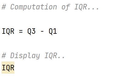
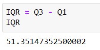
Step 2 : Computation of IQR 

Output - 

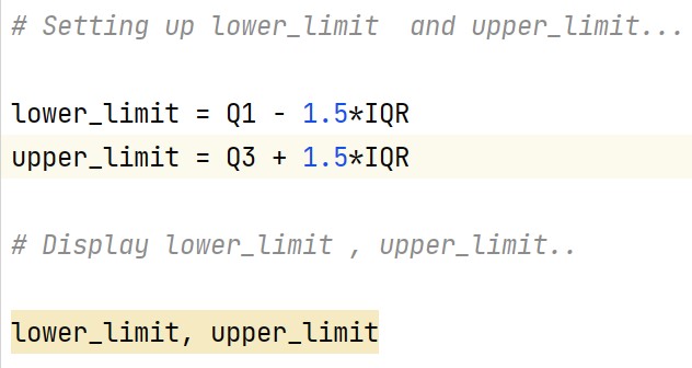
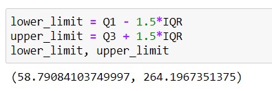
Step 3 : Setting up Lower limit , Upper limit

Output - 

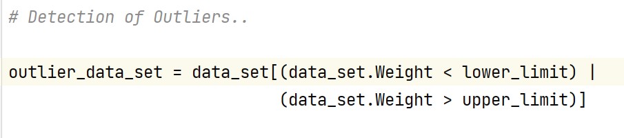
Step 4 : Detection of outliers

As per the condition mentioned, we will make use of lower limit and upper limit for detecting the outliers in the dataset. We create a new dataframe named 'outlier_data_set' which wil used in storing only outliers variables.

 

 

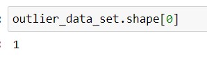
we can have look at shape of dataframe or numbers of outliers present in new dataframe as :

 

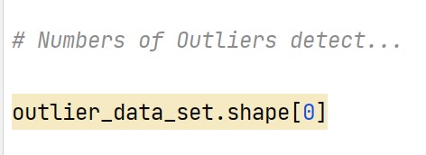
corresponding output - 

Steps for Removal of Outliers ---> using IQR

This step involves the removal of a sub-data frame from the original data frame which thus results in the removal of all outliers from the dataset.

 

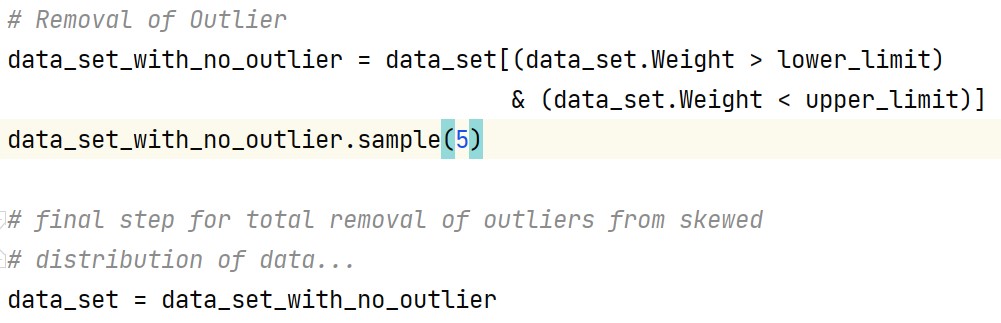
Output - 

 

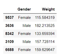
The drawn sample output clearly shows the data values with the condition satisfying for IQR and excluding the remainings(i.e., outliers).

Hence, we have successfully detected and removed the outliers from the dataset.

 

This can be re-verified with the help of visualization of new dataset using histogram plot.

 

Visualization of a new dataset

Code - 

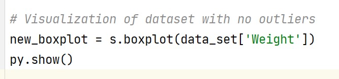
Output - 

hus, here is the final output. You can have a comparison between the two plots and can easily observe the changes that occur after and before consecutively.

 

I HAVE ATTACHED THE FILE CONTAINING THE FORMAT OF THE SOURCE CODE FOR FUTURE USE.