Diabetes detection using Neural Network in Python using Keras
 Saurabh Damle
Nov 04, 2020
Saurabh Damle
Nov 04, 2020
In this project I have built a model in Python with Keras which will detect whether a person has diabetes or not using certain features. Here is a simple ANN to detect diabetes using Keras.
This project is written in Python and will require following libraries:
1.Keras
2.NumPy
3.pandas
4.scikit-learn
5.Seaborn
We will build a neural network which will be able to classify whether a person has diabetes or not.
The steps followed in the project are:
1. Exploring the dataset
2. Data visualization
3. Processing(cleaning) the dataset
4. Building the data pipeline for the model
5. Using keras to build the model and training
6. Model evaluation and tuning.
STEPS:
To begin with, let's import all the libraries.
import tensorflow.keras as keras
import numpy as np
import pandas as pd
from sklearn.model_selection import train_test_split
import os
Let's quickly import the dataset. Here it is in csv format.
ds = pd.read_csv('/content/diabetes.csv')
Then, we will go through the dataset and look at the attributes. As we can see, there are 768 samples, so the dataset is pretty small and it has 8 attributes and the 'Outcomes' column consists of the label - whether the sample has diabetes.
print(ds.info())

<class 'pandas.core.frame.DataFrame'>
RangeIndex: 768 entries, 0 to 767
Data columns (total 9 columns):
 #   Column                    Non-Null Count  Dtype
---  ------                    --------------  -----
 0   Pregnancies               768 non-null    int64
 1   Glucose                   768 non-null    int64
 2   BloodPressure             768 non-null    int64
 3   SkinThickness             768 non-null    int64
 4   Insulin                   768 non-null    int64
 5   BMI                       768 non-null    float64
 6   DiabetesPedigreeFunction  768 non-null    float64
 7   Age                       768 non-null    int64
 8   Outcome                   768 non-null    int64
dtypes: float64(2), int64(7)
memory usage: 54.1 KB
None
Now, let us look at the distribution of the dataset
ds.describe()

Pregnancies 	Glucose 	BloodPressure 	SkinThickness 	Insulin 	BMI 	DiabetesPedigreeFunction 	Age 	Outcome
count 	768.000000 	768.000000 	768.000000 	768.000000 	768.000000 	768.000000 	768.000000 	768.000000 	768.000000
mean 	3.845052 	120.894531 	69.105469 	20.536458 	79.799479 	31.992578 	0.471876 	33.240885 	0.348958
std 	3.369578 	31.972618 	19.355807 	15.952218 	115.244002 	7.884160 	0.331329 	11.760232 	0.476951
min 	0.000000 	0.000000 	0.000000 	0.000000 	0.000000 	0.000000 	0.078000 	21.000000 	0.000000
25% 	1.000000 	99.000000 	62.000000 	0.000000 	0.000000 	27.300000 	0.243750 	24.000000 	0.000000
50% 	3.000000 	117.000000 	72.000000 	23.000000 	30.500000 	32.000000 	0.372500 	29.000000 	0.000000
75% 	6.000000 	140.250000 	80.000000 	32.000000 	127.250000 	36.600000 	0.626250 	41.000000 	1.000000
max 	17.000000 	199.000000 	122.000000 	99.000000 	846.000000 	67.100000 	2.420000 	81.000000 	1.000000
Out of the 8 features, there might be a corelation in between the features, let's check that using a heatmap. Heatmap is used to
import seaborn as sns
import matplotlib.pyplot as plt

def HeatMap(df,x=True):
        correlations = ds.corr()
        ## Create color map ranging between two colors
        cmap = sns.diverging_palette(220, 10, as_cmap=True)
        fig, ax = plt.subplots(figsize=(10, 10))
        fig = sns.heatmap(correlations, cmap=cmap, vmax=1.0, center=0, fmt='.2f',square=True, linewidths=.5, annot=x, cbar_kws={"shrink": .75})
        fig.set_xticklabels(fig.get_xticklabels(), rotation = 90, fontsize = 10)
        fig.set_yticklabels(fig.get_yticklabels(), rotation = 0, fontsize = 10)
        plt.tight_layout()
        plt.show()
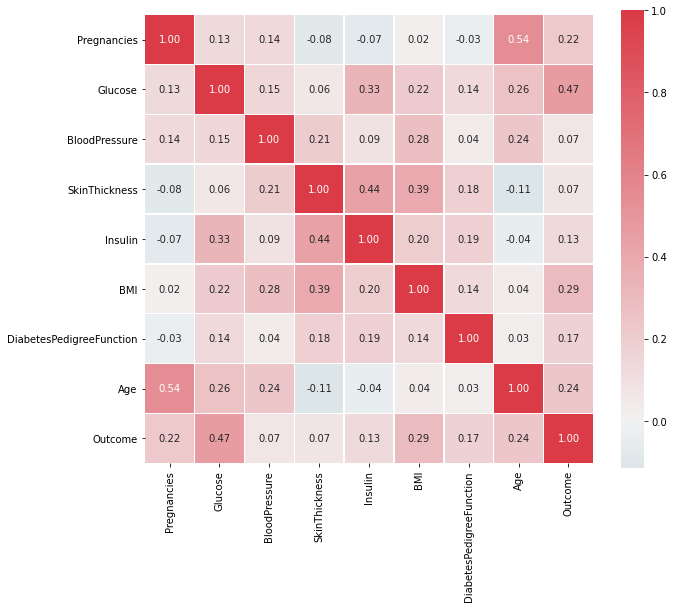
Given the dataset, there is not much of a corelation in the features.
To build the model, lets split it into train and test sets.
input = ds[columns[0:8]]
label = ds[columns[-1]]

x_train, x_test,  y_train, y_test = train_test_split(input, label, train_size=0.8, shuffle=True)
To feed the data into the Neural Network, it should be scaled so it will be computationally easy and it will converge faster.
ip = x_train.values
op = y_train.values

eval_ip = x_test.values
eval_op = y_test.values

from sklearn import preprocessing

scaler = preprocessing.StandardScaler()
ip_scaled = scaler.fit_transform(ip)
eval_ip_scaled = scaler.fit_transform(eval_ip)
Now let's build the model. Here, the input layer has 8 units as we have 8 features, followed by a hidden layer of 1024 units and a output layer of 1 unit. The activation layer used in the output layer is sigmoid as we will have either 0 or 1 as output.
model = keras.Sequential([
                          keras.layers.Dense(8, activation='relu'),
                          keras.layers.Dense(1024, activation='relu'),
                          keras.layers.Dense(1, activation='sigmoid')
])
I have used Stochastic gradient descent as optimizer with learning rate of 0.005 and Binary cross entropy as the loss function
model.compile(optimizer=keras.optimizers.SGD(0.005),metrics='accuracy', loss=keras.losses.BinaryCrossentropy())
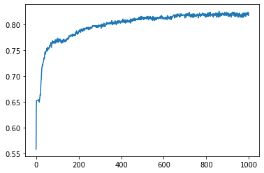
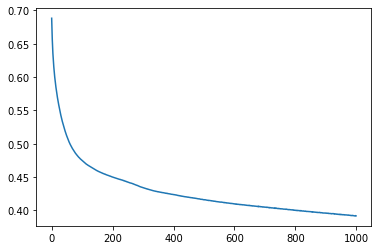
Lets train the model
hist = model.fit(x=ip_scaled, y=op_edims,batch_size=16,epochs=1000)

Epoch 1/1000
39/39 [==============================] - 0s 2ms/step - loss: 0.6881 - accuracy: 0.5586
Epoch 2/1000
39/39 [==============================] - 0s 2ms/step - loss: 0.6701 - accuracy: 0.6368
Epoch 3/1000
39/39 [==============================] - 0s 2ms/step - loss: 0.6563 - accuracy: 0.6531
...
Epoch 1000/1000
39/39 [==============================] - 0s 2ms/step - loss: 0.3916 - accuracy: 0.8225
Here is the summary
model.summary()

Model: "sequential_3"
_________________________________________________________________
Layer (type)                 Output Shape              Param #
=================================================================
dense_17 (Dense)             (None, 8)                 72
_________________________________________________________________
dense_18 (Dense)             (None, 128)               1152
_________________________________________________________________
dense_19 (Dense)             (None, 1)                 129
=================================================================
Total params: 1,353
Trainable params: 1,353
Non-trainable params: 0
_________________________________________________________________
Let's plot the accuracy and the loss
Accuracy
Loss
Project Files
| .. | ||
| This directory is empty. | ||
