Garbage Classification using VGG16 with Keras TensorFlow in the backend

By Amanpreet Singh

The project focuses on classifying garbage scraps such as metals, batteries, paper, and plastic using the VGG16 model.

In this tutorial, we’ll use the VGG16 model with Keras TensorFlow in the backend to try to identify distinct types of garbage scraps, then examine the results to see how the model may be used in practice.

What is VGG16?

A ConvNet is a type of artificial neural network that is also known as a convolutional neural network. An input layer, an output layer, and various hidden layers comprise a convolutional neural network. VGG16 is a CNN (Convolutional Neural Network) that is widely regarded as one of the best computer vision models available today. The creators of this model analyzed the networks and increased the depth with a very small (3*3) convolution filter architecture, which demonstrated a significant improvement over prior-art configurations. They increased the depth to 16-19 weight layers, resulting in approximately 138 trainable parameters.

VGG16 is an image classification algorithm that can classify 1000 images from 1000 different categories with an accuracy of 92.7%. It is a popular image classification algorithm that works well with transfer learning.

The architecture of VGG16 is as follows:

 

 

1. The 16 in VGG16 refers to 16 weighted layers. VGG16 has thirteen convolutional layers, five Max Pooling layers, and three Dense layers in total, for a total of 21 layers, but only sixteen weight layers, i.e., learnable parameters layers.

2. The input tensor size for VGG16 is 224, 244 with three RGB channels.

3. The most distinctive feature of VGG16 is that, rather than having a large number of hyper-parameters, they focused on having convolution layers of 3x3 filter with stride 1 and always used the same padding and max pool layer of 2x2 filter with stride 2.

4. The convolution and max pool layers are arranged consistently throughout the architecture.

5. Conv-1 Layer has 64 filters, Conv-2 Layer has 128 filters, Conv-3 Layer has 256 filters, and Conv 4 and Conv 5 Layers have 512 filters.

6. Following a stack of convolutional layers, three Fully-Connected (FC) layers are added: the first two have 4096 channels each, while the third performs 1000-way ILSVRC classification and thus has 1000 channels (one for each class). The soft-max layer is the final layer.

 

Requirements

In this project, we are using Google Collab IDE with Python version 3.9.In our IDE we need to install certain libraries like :

pip install tensorflow

pip install numpy

pip install Pillow

pip install matplotlib

 

Import Libraries

Let's import all the required libraries which we installed earlier.

import matplotlib.pyplot as plt
import numpy as np
import PIL
import tensorflow as tf
import pathlib
from tensorflow.keras import layers
from tensorflow.keras.models import Sequential
from tensorflow.keras.applications.vgg16 import VGG16
from tensorflow.keras.applications.vgg16 import preprocess_input
import glob
from tensorflow.keras.layers import Input, Lambda, Dense, Flatten,GlobalAveragePooling2D,MaxPooling2D,Dropout
from tensorflow.keras.models import Model
import os

 

Download & Explore Data

First, we need to download the data from the below link.

Garbage Classification Data

When it's downloaded we need to extract Data as the data is in the form of.zip.We can unzip the data by the following command:

!unzip-q {zipfilepath}

Here in our case data is uploaded on  Google Drive. We unzip it by the following:

!unzip -q '/content/drive/MyDrive/archive (2).zip'

After extraction, we need to use the path where data is extracted.

dat_dir=pathlib.Path("/content/Garbage Classification/")

Check Folders & No of Images

Let’s check the number of folders & total no images inside our data directory.

Code

folders = glob.glob('/content/Garbage Classification/*')
print(folders)
#data_dir = data_dir.map(lambda x: tf.image.decode_jpeg(tf.io.read_file(x)))
image_cnt=glob.glob('/content/Garbage Classification/*/*jpg')
print(len(image_cnt))

 

Output

['/content/Garbage Classification/plastic',
'/content/Garbage Classification/metal',
'/content/Garbage Classification/trash',
'/content/Garbage Classification/battery',
'/content/Garbage Classification/paper',
'/content/Garbage Classification/glass',
'/content/Garbage Classification/shoes',
'/content/Garbage Classification/cardboard',
'/content/Garbage Classification/clothes',
'/content/Garbage Classification/biological']
21634

 

 Import Data into Tensorflow Object

Here we are defining the batch size of 32 and image size off 224*224 i.e height, and width.Divide Data into the train, test using

tf.keras.utils.image_dataset_from_directory.Here we take 80% data for training & 20% for validation,
 
Code

batch_size=32
IMG_SIZE=[224,224]
train_ds=tf.keras.utils.image_dataset_from_directory(data_dir,validation_split=0.2,
subset="training",shuffle=True,batch_size=batch_size,
image_size=IMG_SIZE,seed=123)
val_ds=tf.keras.utils.image_dataset_from_directory(data_dir,validation_split=0.2,
subset="validation",shuffle=True,batch_size=batch_size,
image_size=IMG_SIZE,seed=123)

 

Output

Found 21910 files belonging to 10 classes.
Using 17528 files for training.
Found 21910 files belonging to 10 classes.
Using 4382 files for validation.

 

 

Check No of Classes in Data

Let's check the number of classes in our Data

Code

class_names=train_ds.class_names
class_names

 

Output

Here we have a total number of 10 classes.

['battery',
'biological',
'cardboard',
'clothes',
'glass',
'metal',
'paper',
'plastic',
'shoes',
'trash']

 

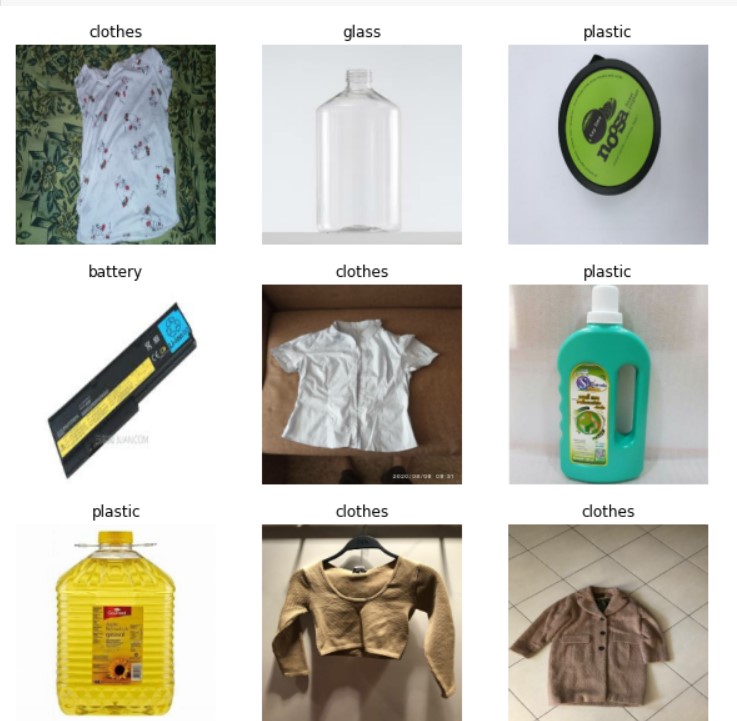
Visualize Image Batch

Let's visualize the first batch of images by the following code

fig=plt.figure(figsize=(10,10))
for img,label in train_ds.take(1):
for i in range(9):
fig.add_subplot(3,3,i+1),plt.imshow(img[i].numpy().astype('uint8'))
plt.title(class_names[label[i]])
plt.axis('off')

Output

 

 Configure Data for Performance

Here, We will create a test set because the original database lacks one. To do so, use tf.data.experimental.cardinality to determine how many data collections are available in the verification set and submit 20% of them to the test set.

Code

## Create Test from valid
val_batches = tf.data.experimental.cardinality(val_ds)
test_dataset = val_ds.take(val_batches // 5)
val_ds = val_ds.skip(val_batches // 5)

print('Number of validation batches: %d' % tf.data.experimental.cardinality(val_ds))
print('Number of test batches: %d' % tf.data.experimental.cardinality(test_dataset))
print('Number of train batches: %d' % tf.data.experimental.cardinality(train_ds))

 

Output

Number of validation batches: 110
Number of test batches: 27
Number of train batches: 548

 

Now, make use of buffered prefetching so that you can retrieve data from the disc without I/O becoming blocked. When loading data, you should use the following two methods:

After the images are loaded from the disc during the first epoch, Dataset.cache keeps them in memory. This will prevent the dataset from becoming a bottleneck while training your model. If your dataset is too large to fit in memory, you can use this method to build a fast on-disk cache.
While training, Dataset.prefetch overlaps data preprocessing and model execution.

Code

AUTOTUNE = tf.data.AUTOTUNE
train_ds = train_ds.prefetch(buffer_size=AUTOTUNE)
val_ds = val_ds.prefetch(buffer_size=AUTOTUNE)
test_dataset = test_dataset.prefetch(buffer_size=AUTOTUNE)

Apply Data Augmentation to Dataset

Here first we generate a new random sample of training data that includes image rotation and horizontal flipping, then we visualize our augmented image results with the help of matplotlib library.

Code

data_augmentation = tf.keras.Sequential([
tf.keras.layers.RandomFlip('horizontal'),
tf.keras.layers.RandomRotation(0.2),
])

plt.figure(figsize=(10, 10))
for images, _ in train_ds.take(1):
for i in range(9):
augmented_images = data_augmentation(images)
ax = plt.subplot(3, 3, i + 1)
plt.imshow(augmented_images[0].numpy().astype("uint8"))
plt.axis("off")

 

Output

Model Building

The model-building stage consists of :

1. Create the Model.

2. Compile the Model.

3. Train the Model.

4. Model Fine Tunning (if required)

5. Evaluate Model.

6. Make Predictions.

Create the Model

To begin, create a VGG16 model that has been pre-loaded with ImageNet weights. Bypassing the include top=False argument, you can load a network without the classification layers at the top, which is ideal for feature extraction.

Code

IMG_SHAPE = IMG_SIZE + [3]
base_model=VGG16(input_shape=IMG_SHAPE,include_top=False,weights='imagenet')

 

Output

Downloading data from https://storage.googleapis.com/tensorflow/keras-applications/vgg16/vgg16_weights_tf_dim_ordering_tf_kernels_notop.h5
87916544/87910968 [==============================] - 1s 0us/step
87924736/87910968 [==============================] - 1s 0us/step
Model: "VGG16"

 

Before assembling and training the model, it is critical to establish a convolutional base. By setting layer. trainable = False, you can prevent weight loss in a specific layer from being repeated during training. Because Inception V3 has many layers, setting the trainable flag for the entire model to False will freeze all of them.

#Freeze the layers in the base model
base_model.trainable=False

 

When you enable it, the batch normalization layer enters inference mode and does not update its mean and variance statistics.

Using the Keras Functional API, we now create a model by combining data augmentation, re-scaling, base model, and feature extraction layers. As previously stated, because our model contains the BatchNormalization layer, use training = False.

Code

inputs=base_model.input
x=data_augmentation(inputs)
x=preprocess_input(x)
x=base_model(x, training=False)
x=global_average_layer(x)
x=Dropout(0.2)(x)
outputs=Dense(len(folders), activation='softmax')(x)
model = Model(inputs, outputs)
model.summary()

Output

Model: "model_2"
_________________________________________________________________
Layer (type) Output Shape Param #
=================================================================
input_3 (InputLayer) [(None, 224, 224, 3)] 0

sequential_3 (Sequential) (None, 224, 224, 3) 0

tf.__operators__.getitem_2 (None, 224, 224, 3) 0
(SlicingOpLambda)

tf.nn.bias_add_2 (TFOpLambd (None, 224, 224, 3) 0
a)

vgg16 (Functional) (None, 7, 7, 512) 14714688

global_average_pooling2d_3 (None, 512) 0
(GlobalAveragePooling2D)

dropout_2 (Dropout) (None, 512) 0

dense_3 (Dense) (None, 10) 5130

=================================================================
Total params: 14,719,818
Trainable params: 5,130
Non-trainable params: 14,714,688

Compile the Model

Before training the model, compile it. Because there are 10 classes, use the following:

. Select optimizer = Adam(Momentum+RMS Prop) as it is most used by industry experts.
. Select loss= Sparse Categorical.
. Select metrics= ‘accuracy’ (can choose any other metrics like precision, recall, f1-score, etc depending on the problem)

Train the model for 10 epochs with the Keras Model.fit method.

Code

base_learning_rate = 0.0001
model.compile( optimizer=tf.keras.optimizers.Adam(learning_rate=base_learning_rate),
loss=tf.keras.losses.SparseCategoricalCrossentropy(from_logits=False),
metrics=['accuracy'] )
history = model.fit(train_ds, epochs=10, validation_data=val_ds)

 

Output

Epoch 1/10
548/548 [==============================] - 126s 227ms/step - loss: 4.9363 - accuracy: 0.2697 - val_loss: 2.4588 - val_accuracy: 0.4892
Epoch 2/10
548/548 [==============================] - 125s 227ms/step - loss: 2.2573 - accuracy: 0.5295 - val_loss: 1.3351 - val_accuracy: 0.6808
Epoch 3/10
548/548 [==============================] - 125s 227ms/step - loss: 1.5881 - accuracy: 0.6389 - val_loss: 0.9515 - val_accuracy: 0.7564
Epoch 4/10
548/548 [==============================] - 125s 227ms/step - loss: 1.2526 - accuracy: 0.7020 - val_loss: 0.7556 - val_accuracy: 0.7996
Epoch 5/10
548/548 [==============================] - 125s 228ms/step - loss: 1.0490 - accuracy: 0.7387 - val_loss: 0.6367 - val_accuracy: 0.8246
Epoch 6/10
548/548 [==============================] - 126s 228ms/step - loss: 0.9111 - accuracy: 0.7657 - val_loss: 0.5471 - val_accuracy: 0.8474
Epoch 7/10
548/548 [==============================] - 125s 226ms/step - loss: 0.8234 - accuracy: 0.7837 - val_loss: 0.4932 - val_accuracy: 0.8644
Epoch 8/10
548/548 [==============================] - 126s 229ms/step - loss: 0.7474 - accuracy: 0.7993 - val_loss: 0.4605 - val_accuracy: 0.8738
Epoch 9/10
548/548 [==============================] - 126s 229ms/step - loss: 0.6729 - accuracy: 0.8140 - val_loss: 0.4280 - val_accuracy: 0.8789
Epoch 10/10
548/548 [==============================] - 127s 230ms/step - loss: 0.6418 - accuracy: 0.8181 - val_loss: 0.4047 - val_accuracy: 0.8835

 

If you're curious why validation metrics are superior to training metrics, it's because of layers like tf.keras.layers.Dropout and tf.keras.layers. BatchNormalization. Dropout has an impact on accuracy during training. When calculating validation loss, they are disabled.

Fine-Tune Model

Train (or "fine-tune") the weights of the top layers of the pre-trained model alongside the training of the classifier you added to improve performance even further. The weights will be forced to be tuned from generic feature maps to features specific to the dataset during the training process.

Simply unfreeze the base model and set the bottom layers to un-trainable. Then, recompile the model (which is required for these changes to take effect) and resume training.

Code

base_model.trainable=True
# Let's take a look to see how many layers are in the base model
print("Number of layers in the base model: ", len(base_model.layers))

# Fine-tune from this layer onwards
fine_tune_at = 10

# Freeze all the layers before the `fine_tune_at` layer
for layer in base_model.layers[:fine_tune_at]:
layer.trainable = False

 

Output

Number of layers in the base model: 19

 

Compile & Train Fine-Tuned Model

Because we are training a much larger model and want to readapt the pre-trained weights, a lower learning rate is required at this stage. Otherwise, your model may quickly overfit.

If you previously trained to convergence, this step will increase your accuracy by a few percentage points.

base_learning_rate = 0.0001
model.compile( optimizer=tf.keras.optimizers.Adam(learning_rate=base_learning_rate/10),
loss=tf.keras.losses.SparseCategoricalCrossentropy(from_logits=False),
metrics=['accuracy'] )
initial_epochs = 10
fine_tune_epochs = 10
total_epochs = initial_epochs + fine_tune_epochs

history_fine = model.fit(train_ds,
epochs=total_epochs,
initial_epoch=history.epoch[-1],
validation_data=val_ds)

 

Output

Epoch 10/20
548/548 [==============================] - 169s 302ms/step - loss: 0.4419 - accuracy: 0.8594 - val_loss: 0.2695 - val_accuracy: 0.9153
Epoch 11/20
548/548 [==============================] - 166s 300ms/step - loss: 0.2893 - accuracy: 0.9056 - val_loss: 0.2084 - val_accuracy: 0.9312
Epoch 12/20
548/548 [==============================] - 165s 301ms/step - loss: 0.2132 - accuracy: 0.9292 - val_loss: 0.2109 - val_accuracy: 0.9392
Epoch 13/20
548/548 [==============================] - 165s 301ms/step - loss: 0.1766 - accuracy: 0.9420 - val_loss: 0.1993 - val_accuracy: 0.9474
Epoch 14/20
548/548 [==============================] - 165s 300ms/step - loss: 0.1484 - accuracy: 0.9496 - val_loss: 0.1717 - val_accuracy: 0.9531
Epoch 15/20
548/548 [==============================] - 167s 303ms/step - loss: 0.1237 - accuracy: 0.9591 - val_loss: 0.2101 - val_accuracy: 0.9426
Epoch 16/20
548/548 [==============================] - 165s 300ms/step - loss: 0.1041 - accuracy: 0.9672 - val_loss: 0.2256 - val_accuracy: 0.9363
Epoch 17/20
548/548 [==============================] - 165s 301ms/step - loss: 0.0936 - accuracy: 0.9687 - val_loss: 0.1938 - val_accuracy: 0.9531
Epoch 18/20
548/548 [==============================] - 165s 301ms/step - loss: 0.0832 - accuracy: 0.9718 - val_loss: 0.1552 - val_accuracy: 0.9548
Epoch 19/20
548/548 [==============================] - 166s 302ms/step - loss: 0.0729 - accuracy: 0.9752 - val_loss: 0.1809 - val_accuracy: 0.9559
Epoch 20/20
548/548 [==============================] - 166s 302ms/step - loss: 0.0620 - accuracy: 0.9795 - val_loss: 0.2089 - val_accuracy: 0.9466

 

Visualize Training Result

Let's look at the training and validation accuracy/loss learning curves when fine-tuning the last few layers of the VGG16 base model and training the classifier on top of it.

After fine-tuning, the model nearly reaches 95% accuracy on the validation set.

Code

acc += history_fine.history['accuracy']
val_acc += history_fine.history['val_accuracy']

loss += history_fine.history['loss']
val_loss += history_fine.history['val_loss']
plt.figure(figsize=(8, 8))
plt.subplot(2, 1, 1)
plt.plot(acc, label='Training Accuracy')
plt.plot(val_acc, label='Validation Accuracy')
plt.ylim([0.8, 1])
plt.plot([initial_epochs-1,initial_epochs-1],
plt.ylim(), label='Start Fine Tuning')
plt.legend(loc='lower right')
plt.title('Training and Validation Accuracy')

plt.subplot(2, 1, 2)
plt.plot(loss, label='Training Loss')
plt.plot(val_loss, label='Validation Loss')
plt.ylim([0, 1.0])
plt.plot([initial_epochs-1,initial_epochs-1],
plt.ylim(), label='Start Fine Tuning')
plt.legend(loc='upper right')
plt.title('Training and Validation Loss')
plt.xlabel('epoch')
plt.show()

 

Output

Evaluate Model 

Let's evaluate our model on test data.

Code

loss, accuracy = model.evaluate(test_dataset)
print('Test accuracy :', accuracy)

 

Output

27/27 [==============================] - 5s 155ms/step - loss: 0.2450 - accuracy: 0.9306
Test accuracy : 0.9305555820465088