Predicting car prices by linear regression using scikit-learn in Python

By Saurabh Damle

This project is demonstration of simple linear regression in Python using scikit-learn on real world problem of predicting car prices.

This project is written in python and uses following libraries:

1. NumPy

2. pandas

3.Seaborn

4.scikit-learn

5. Matplotlib.

In this project, we will be using linear regression to build model which will be used to predict resale value of cars. The dataset used in the model is from Car-Dekho website.

The steps followed in the project are:

1. Exploring the dataset

2. Data visualization

3. Processing(cleaning) the dataset

4. Building the data pipeline for the model

5. Using sklearn to build the model and training

6. Model evaluation and tuning.

STEPS:

To begin with, we will first import all the required libraries

import numpy as np
import pandas as pd
import seaborn as sns
import matplotlib.pyplot as plt

Then we will import the dataset

df = pd.read_csv('/content/CAR DETAILS FROM CAR DEKHO.csv')

Let's have a look at the dataset. As we can see, it has several factors like year, total kilometers driven, transmission type, etc which we will be using to build the model.

df.head()


  year 	selling_price 	km_driven 	fuel 	seller_type 	transmission 	owner
0 	2007 	60000 	70000 	Petrol 	Individual 	Manual 	First Owner
1 	2007 	135000 	50000 	Petrol 	Individual 	Manual 	First Owner
2 	2012 	600000 	100000 	Diesel 	Individual 	Manual 	First Owner
3 	2017 	250000 	46000 	Petrol 	Individual 	Manual 	First Owner
4 	2014 	450000 	141000 	Diesel 	Individual 	Manual 	Second Owner


df.info()

<class 'pandas.core.frame.DataFrame'>
RangeIndex: 4340 entries, 0 to 4339
Data columns (total 8 columns):
 #   Column         Non-Null Count  Dtype 
---  ------         --------------  ----- 
 0   name           4340 non-null   object
 1   year           4340 non-null   int64 
 2   selling_price  4340 non-null   int64 
 3   km_driven      4340 non-null   int64 
 4   fuel           4340 non-null   object
 5   seller_type    4340 non-null   object
 6   transmission   4340 non-null   object
 7   owner          4340 non-null   object
dtypes: int64(3), object(5)
memory usage: 271.4+ KB

processed_df = df[['year', 'selling_price','km_driven','fuel', 'seller_type', 'transmission', 'owner']]

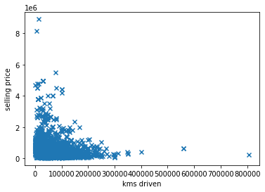
Lets's visualize the data to find correlations

plt.scatter(x=df['km_driven'], y=df['selling_price'], marker='x')
plt.xlabel('kms driven')
plt.ylabel('selling price')
plt.show()

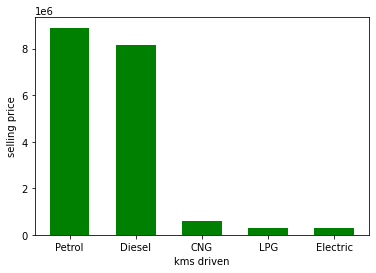
plt.bar(df['fuel'], df['selling_price'], width=0.6, color='green')
plt.xlabel('kms driven')
plt.ylabel('selling price')
plt.show()

There are some non numeric features that need to be converted to numeric values for processing.

processed_df = pd.get_dummies(processed_df,columns=['fuel','transmission','seller_type','owner'],drop_first=True)

Next, let's generate a heatmap to find correlations. If there are features with high correlation, we will drop one of them.

correlations = processed_df.corr()

indx=correlations.index
plt.figure(figsize=(20,15))
sns.heatmap(processed_df[indx].corr(),annot=True,cmap="YlGnBu")

*unfortunately I am unable to upload the image due to dimension constraints, but you can access it in the notebook

Now, we will create the input matrix(independant variables) and the output value which is the price(dependant variable)

data = processed_df.values
x = data[:,2:14]
y = data[:,1]

Next, we will scale down the input matrix so that computation becomes quick and it takes less time to converge. Here we will be using a standard scaler to scale the values.

x = preprocessing.StandardScaler().fit(x).transform(x.astype(float))

x

[[ 0.08113906 -0.99219635 -0.01518117 ... -0.58480026 -0.06270928
  -0.27444872]
 [-0.3476891  -0.99219635 -0.01518117 ... -0.58480026 -0.06270928
  -0.27444872]
 [ 0.7243813   1.00786503 -0.01518117 ... -0.58480026 -0.06270928
  -0.27444872]
 ...
 [ 0.35987736 -0.99219635 -0.01518117 ...  1.70998557 -0.06270928
  -0.27444872]
 [ 0.50996722  1.00786503 -0.01518117 ... -0.58480026 -0.06270928
  -0.27444872]
 [-0.56210318 -0.99219635 -0.01518117 ... -0.58480026 -0.06270928
  -0.27444872]]

Now, we will split the data into train and test sets.

from sklearn.model_selection import train_test_split
train, test, train_price, test_price = train_test_split(x,y, test_size = 0.05) 

Now, let us build the model. For this we will be using linear regression. We will be using polynomial features of degree two for this model.

from sklearn import linear_model
from sklearn.metrics import r2_score
from sklearn.preprocessing import PolynomialFeatures

second_order = PolynomialFeatures(2)
train_order_2 = second_order.fit_transform(train)

lr_2 = linear_model.LinearRegression()
lr_2.fit(train_order_2, train_price)

test_order_2 = second_order.fit_transform(test)
y_hat_2 = lr_2.predict(test_order_2)

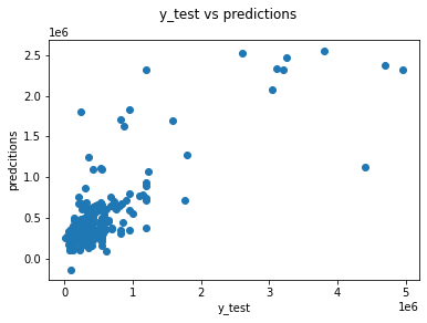
Let's look at r squared score. We are getting a r2 score of 0.61

r2_score(test_price,y_hat_2)
0.6168079383911376

Let's plot the predictions. We can see the plot of actual values of the x-axis and predicted values on the y axis. So the model performs decently.

fig = plt.figure()
fig.suptitle('y_test vs predictions')
plt.xlabel('y_test')
plt.ylabel('predcitions')
plt.scatter(test_price,y_hat_2)